Discount Rates, Natural Resource Damages, and the Public Trust

1. Introduction

When unpermitted releases of contamination to the environment cause injuries to natural resources in the United States, various federal and state environmental liability statutes allow the recovery of monetary natural resource damages (NRDs) from the parties whose releases caused the injury. NRDs are estimated by government agencies acting on behalf of the public as trustees for natural resources. NRDs collected are then spent on natural resource restoration projects that provide sufficient benefits to redress the harms.

The sufficiency of compensatory restoration is determined in the natural resource damage assessment (NRDA) process by quantifying injury to resources (an ecological “debit”) and the benefits of restoration (a “credit”). The debits and credits represent changes in public wellbeing resulting from changes in the natural resource services provided by resources. In a typical NRDA (and especially for contaminated sites), these debits and credits are experienced over large expanses of time. A discount rate is used to convert debits or credits occurring at different points in time to a common unit at a single point in time (the “base year,” usually when the claim is presented) so they can be added together as a present value total. Restoration is deemed sufficient to compensate the public when the discounted credit it generates meets or exceeds the discounted debit incurred.

The expansive economic literature on the discount rate typically is couched in terms of benefit-cost analysis (BCA) of public investment projects. Current practice in NRDA relies on this literature to specify one discount rate to apply to all elements of the assessment. As a result, and as explained further below, a 3% discount rate is applied as a default rate to all elements of essentially every NRDA.

However, NRDA has two features that make it different than BCA, which may undermine the adoption of the BCA discount rate. First, NRDA has a backward-looking component that BCA does not, with past injury compounded forward to the base year. This raises some issues, discussed below, related to changing public preferences, observation of the past versus forecasting the future, and compensation of persons no longer alive.

Second, BCA places all sources of impact on public wellbeing on equal footing—if a project fails a benefit-cost test, it means that there is some other unidentified expenditure of the project’s costs (all costs are opportunity costs) that could provide more benefit to the public than the project. Moreover, costs and potential benefits are denominated in a common unit so they can be compared. This common unit is a generalized aggregate consumption good. Idealized prices are used to convert all pluses and minus from the project to consumption equivalents. The discount rate is applied to these consumption equivalents in BCA. As a consequence of this aggregation of all effects via prices, there is only one discount rate, a consumption rate of discount that would be applied to all projects. This measures the public’s willingness to trade units of generalized consumption across time.

The consumption rate of discount is also called the social rate of time preference (SRTP), but one needs to be careful here. The concept of a SRTP could apply to any good or service. It is usually implicit that consumption goods are the entities of interest (BCA thinking) and so the SRTP equates to the consumption rate of discount. But one might also think of a SRTP for ecological services. Henceforth, I will use the term SRTP narrowly to refer to a discount rate for aggregate consumption.

The translation to consumption equivalents with prices is manifestly different than NRDA, where compensatory restoration supplies ecological services for each resource separately. An injury to shoreline fishing may be compensated by a fishing pier, injury to birds compensated by nest protection, and injury to sediments compensated by a wetlands project, and so on. Further, these services typically are not monetized (except for recreation trips) but are quantified in natural service units. What is needed is an ecological service discount rate (ESDR).

There is no a priori reason to think that one discount rate, and especially one drawn from the BCA context, would apply to all the elements of NRDA. This paper addresses this issue. It emerges that there are, in principle, many ESDRs, potentially different for each resource, for different time periods, and for each case’s site-specific facts.

Rather than a fixed number for all cases that does not warrant further discussion once established, the ESDR in this view is much like other aspects of the assessment of debits and credits over time that routinely are estimated using scientific and economic analyses particular to each case.

2. The Importance of the Discount Rate

The numerical value of the discount rate has an outsized impact on the magnitude of estimated NRDs. Let 𝑑 be the annual percentage rate of discount (the ESDR, assumed constant for now). A change in public wellbeing of size ∆𝑊 occurring 𝑡 years before the base year (e.g., a past debit) has a present value equivalent change in the base year calculated as ∆𝑊 × (1 +𝑑)^t. Thus, past effects are compounded forward at the rate 𝑑 and increase exponentially with the time span. At a 3% discount rate, a 100-unit change in 1980 compounded forward to a base year of 2022 is worth 346 units. A service change of this same amount occurring 𝑡 years after the base year (e.g., a future credit) is equivalent to ∆𝑊 ÷(1 + 𝑑)^t units of service change in the base year, a quantity that shrinks exponentially with the time span. At a 3% discount rate, a 100-unit change in 2044 discounted back to 2022 is worth 27.2 units.

Imagine a NRDA begins in 2022 and takes 9 years to complete, so the base year is 2031. Under the Comprehensive Environmental Response, Compensation and Liability Act (CERCLA), injuries begin to accrue as of December 1980, so 50 years of injury is compounded forward to 2031. If restoration starts in 2032 and lasts 75 years, all told, effects on services in this scenario span 125 years—fully four generations! The exponential feature of discounting and the long spans of time over which it operates in NRDA combine to imply that the discount rate is an extremely important parameter in NRDA calculations.

To see how significant the impact might be, assume the injury in the above example is constant from 1981 to 2031 and that restoration instantaneously provides a constant uplift. The difference between a 3% discount rate and a 1% discount rate is a factor of 2.7, with a $60 million dollar claim using the higher rate changing to a $22.5 million dollar claim using the lower one. Of course, a rate greater than 3% would raise NRDs above $60 million. Multiple tens of millions of NRDs ride on small changes in this single parameter. It is an understatement to say it is important to get it right.

A “default” discount rate of 3% is applied in essentially all NRDAs. Three questions are immediately begged. First, what is the basis for the 3% rate and is it appropriately applied in NRDA? Second, when the basis does apply, is 3% the right number? And third, if either or both of the first two questions are answered “no,” what rates would be more appropriate? Before turning to these questions, it is important to gain a common understanding of what a discount rate is.

3. What are Discount Rates?

Imagine you find that 2 of your last 3 eggs have gone bad when your larder is bare and you were counting on those eggs for a breakfast for two. This is an entirely different event than if you find those eggs bad when you have another dozen good eggs in the fridge. Finding a bad egg (or discovering another good one) has a different impact on your wellbeing in those alternative circumstances. Suppose a benevolent egg fairy appears who wishes to compensate you for your 2-egg loss by providing a benefit of 𝐵 more eggs a day hence, after you have been to the store and have a dozen eggs on hand. Each compensatory egg (received when you will be flush with eggs) generates less incremental wellbeing than those gone bad (lost when eggs were dear). As a consequence, the fairy understands that more than 2 compensatory eggs are needed to make you whole.

Moreover, the egg fairy saw you drumming your fingers on the countertop at the prospect of waiting for your compensatory eggs. Due to this impatience, you may need more compensatory eggs in the future to replace those lost now because, from today’s perspective, a frittata in the future is just not as highly valued as a frittata today, independent of the number of baseline eggs you have at the time.

The discount rate in the example is defined by how many more eggs you to need to feel compensated than the number lost today. Specifically, if 𝐶 is the number of eggs lost (a cost equal to 2 in this example) and 𝐵 is the compensation (a benefit), the one-period discount rate is defined by the equation 𝐶 = 𝐵 ÷ (1 + 𝑑). If the fairy (both benevolent and omniscient) divines that 3 eggs will make you whole, then 𝑑 = (3⁄2)− 1, and your daily discount rate for eggs is revealed to be 50%.

This fanciful example is useful because it uncovers universally applied principles, independent of financial aspects of interest rates based on money, banks, savings rates, and so on. In NRDA, in place of eggs we have natural resource services, and in place of enjoyment derived from a breakfast with a friend, we have public wellbeing derived from nature’s services. And, of course, the Trustees must replace the egg fairy, and develop a theory and empirical methods with which to estimate the ESDR.

Pick a fixed amount of ecological service change (∆𝑆) and call this one unit (the equivalent of 1 egg). Pick a base year (call this year 0), and label the change in public wellbeing from ∆𝑆 in the base year ∆𝑊₀ . Now, compute the change in same wellbeing measure, from the same fixed change in services ∆𝑆, at points in time other than the base year. As above, time is measured as the number of years (𝑡) before or after the base year. Call these out-year measures of changed wellbeing ∆𝑊_𝑡 . If ∆𝑊_𝑡 is different than ∆𝑊₀ , a non-zero discount rate is needed to make these equal. This rate is the ESDR, 𝑑_𝑡 . It depends on the time differential, among other things, and so has a time subscript on it.

The egg example stresses two reasons why the ratio of ∆𝑊_𝑡 to ∆𝑊₀ might change over time: 1) the public’s rate of impatience, and/or 2) changes in the baseline level of services from which the change in services is measured. These two considerations are encapsulated in the expression:

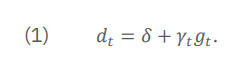
The term 𝛿 captures impatience—if a unit of wellbeing (𝑊) is experienced further in the future, its relative impact, viewed from today, declines at the annual percentage rate 𝛿 . Whether 𝛿 is constant or not is a subject of recent investigation. This term may also represent uncertainty about whether one will be alive in future to receive the benefit. I discuss these issues below.

The term 𝛾_𝑡𝑔_𝑡 is the baseline effect. The parameter 𝛾_𝑡 is the rate at which changes in wellbeing from NRDA debits and credits are responsive to the baseline level of services. It is akin to how you feel about a 1-egg loss or gain depending on whether you have 3 or 12 eggs at baseline. The term 𝑔_𝑡 is the rate of change through time in the baseline quantity of the service that is being lost via injury or gained via restoration. It is akin to whether you had 3 eggs or 12 at the time of loss and gain.

Both terms have a time subscript because they generally vary through time. How the discount rate 𝑑_𝑡 varies with time is called the “term structure” of the discount rate; the 3% rate is constant, having a “flat” term structure and therefore comes from a special model of discount rates.

Thus far, I have reached

Conclusion 1: Discount rates measure a person’s indifferent rate of trade of something across time—a willingness to give up one unit of something today for an amount of that something in the future that just compensates for today’s loss. Discount rates account for two factors: i) impatience, and ii) that a person may have more or less of the thing being traded in the future than they possess today, rendering future compensatory increments relatively more or less valuable than today’s loss. Discount rates generally will depend both on what is being traded through time and the time span associated with the trade.

4. The “Default” 3% NRDA Discount Rate

4.1 The Stated Basis of the 3% Discount Rate in NRDA

How does the 3% discount rate ubiquitous in NRDA relate to the notions elucidated above? As explained by Dunford (2018) and summarized below, the 3% NRD rate has been justified based on indirect observations of the rate of trade across time of the consumption of a generalized bundle of market goods in the economy (approximately the level of the Gross Domestic Product [GDP]). Thus, it is an estimate of the SRTP, derived from BCA thinking.

As in the example where baseline eggs went from 3 to 12, the economy in the U.S. has been growing steadily over time. A public investment may divert consumption to a project now (a cost) in return for an increase in consumption later (a benefit). Due to economic growth, the cost is incurred when consumption is relatively low (and worth relatively more per unit) and benefits conferred when consumption is relatively high (and worth relatively less per unit). Because each future unit of consumption benefit is worth less than today’s cost, more future benefits must be provided than are invested now to make the public whole. That is, the rate of discount for consumption goods is positive. This is without impatience, which only adds to the effect.

The canonical model of the discount rate in BCA shows that in a market equilibrium, rational consumers will set their indifferent rate of trade of consumption through (the SRTP) time equal to the rate of return on investments in the economy, which I will denote by 𝑟_𝑡 . The SRTP is not directly observable, but the rate of return to investment is. The market equilibrium equates the two and thereby reveals the SRTP—in this case, the “magic of the marketplace” takes the place of the egg fairy.

The SRTP is a consumption rate of discount, reminding us that it applies to aggregate consumption. This is distinguished from the rate of impatience, 𝛿, which applies to wellbeing, and is often called the utility rate of discount. These distinctions reveal an important point for NRDA: the discount rate differs according to exactly what it is that is being discounted. On this basis, the SRTP is, in principle, distinct from the ESDR, which applies to ecological services, not aggregate consumption.

Using the exact same reasoning as above that led to equation (1), but now applied to consumption goods instead of nature’s services, the public’s SRTP equals 𝛿 + 𝛽_𝑡𝑐_𝑡 . In market equilibrium,

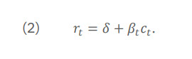
This is a famous equation called the Ramsey equation. It clearly is similar to the ESDR equation 𝑑_𝑡 = 𝛿 +𝛾_𝑡𝑔_𝑡 . The utility rate of discount 𝛿 is the same in both expressions. The term 𝛽_𝑡  in the SRTP captures how increments to wellbeing from increments in consumption depend on the level of baseline consumption, analogous to 𝛾_𝑡 for ecological services. And the term 𝑐_𝑡  in the SRTP is the growth rate of the overall economy (aggregate consumption) through time, analogous to 𝑔_𝑡  for ecological services.

The beauty of the Ramsey equation for BCA is that 𝑟_𝑡  is observable empirically. Hence, if we wanted to use the SRTP in NRDA, we set the discount rate equal to the rate of return on investments (𝑑_𝑡 = 𝑟_𝑡). This is the theoretical basis for the 3%. However, in NRDA we don’t want the SRTP, we want the ESDR. When would these be equal so that the latter is well-measured by the former?

The vital insight for the theoretical legitimacy of 3% is that the ESDR equals the SRTP if 𝛾_𝑡𝑔_𝑡 = 𝛽_𝑡𝑐_𝑡 . That is, the BCA discount rate can reasonably be applied in NRDA: 1) if society cares about the enjoyment of nature’s services exactly as it cares about consumption of market goods ( 𝛾_𝑡 = 𝛽_𝑡 ), and 2) if baseline ecological services are changing over time at the same rate as economic growth ( 𝑔_𝑡 = 𝑐_𝑡 ). Without further analysis, there is no particularly good reason to think that either of these will hold, even approximately, except by serendipity, a poor basis for specifying an important NRDA parameter.

As an aside, the market equilibrium relationship 𝑟_𝑡 = 𝛿 + 𝛽_𝑡𝑐_𝑡 that reveals the public’s SRTP is based on a model economy with well-functioning markets inhabited by rational actors. However, the market data we observe represents the choice behavior of the public and managers of firms—which may exhibit whatever behavioral anomalies real people exhibit—and equilibrium in markets that exhibit whatever market imperfections that real markets embody. I raise this issue now and return to it below where I examine the relevance of market information for decisions made regarding public trust resources.

To summarize, I have reached

Conclusion 2: The discount rate depends on what is being discounted (Conclusion 1). The 3% default rate is based on the SRTP, which discounts consumption, and a market equilibrium that equates the SRTP to a market rate of return to investments. This is conceptually different than the ESDR for use in NRDA, which discounts natural resource services. The two may be equal if their determinants are equal, but this will be true only by happenstance—when we care about resources just the way we care about consumption and when natural resource services change over time the same way as the entire economy grows or shrinks over time.

4.2 Empirical Estimation of the 3% Discount Rate

Turning to the estimation of the 3% rate, there are many rates of return in the economy. We want a risk-free rate for NRDA because we handle risk directly in the assessment of gains and losses, and to employ a risky rate of return would lead to a double-counting of the effects of uncertainty. Therefore, if we are to use a market-revealed SRTP in NRDA, the 𝑟_𝑡  we observe should be a risk-free rate of return. A good estimate of the risk-free rate is the return on holding short-term government securities. The primary justification for the 3% rate is based on data on the real (taking out inflation) annual rate of return to 3-month U.S. Treasury Bills (as risk-free as one can get). At the time when the 3% rate was being justified (the late 1990s), these data showed that the average return for the prior 15 years was about 3% (NOAA 1999). There you have it!

An immediate question is whether this time period is representative. It is not. Updating the data for the average rate on 3-month Treasury Bills between 1981 and 2022 yields a 1% average rate. This would seem to apply to past events at CERCLA sites. For future effects, perhaps a better forecast is the average rate over a very long time period, incorporating many economic upswings and downturns, say from 1900 to 2022. This average is also 1%. Hence, 3% seems an empirical anomaly using the very reasoning that generated it.

Thus, I can state

Conclusion 3: Suppose the SRTP is to be used in NRDA, and a risk-free market rates of return to investment are sued to estimate it. The 3% number for the SRTP was estimated in 1999 from the prior 15 years of data, which was a historically unusual period. Updating the data to today, it is more like 1%, also equal to the long-term average over many business cycles.

However, this mechanical updating of empirical measurement using the original logic behind the 3% (using the SRTP in NRDA) bypasses two deeper questions that I address in turn.

5. Two Deeper Questions

5.1 Deeper Question 1: Should the Consumption Rate of Discount (SRTP) Be Used in NRDA?

The first deeper question is whether the BCA / SRTP reasoning behind the 3% rate should ever be applied in NRDA; after all in NRDA, trades across time are in units of ecological services, not consumption of market goods as in the SRTP. Looked at another way, can we legitimately set the ecological discount rate (𝑑) equal to the consumption rate of discount (𝑆𝑅𝑇𝑃 = 𝑟) because they have the same determinants (𝛾𝑔 = 𝛽𝑐)? The answer depends on the restoration scaling model being used for the
resource at hand, which boils down to whether we are using a valuation approach, as is typical for assessing recreation services, or service-based metrics, as is typical for assessing ecological services of habitats and individual resources.

5.1.1 Recreation

The basic economic model of recreation used in NRDAs has two goods: an aggregate consumption good and recreation trips. Therefore, to assess the applicability of the SRTP, the Ramsey equation needs to consider these same two goods.

The single aggregate consumption good in the Ramsey model can be interpreted as a composite of many market goods, added up by weighting with idealized prices. These are “shadow prices” reflecting well-functioning markets and a socially optimal distribution of income across persons alive at one time (a “generation”). The “price” of the overall aggregate is normalized to $1; the composite consumption good corresponds to the macroeconomic idea of national income (roughly GDP).

The whole point of NRDA (which is based on microeconomic analysis) is that recreation is unbundled from this aggregate consumption good. Otherwise, compensatory payments made in money would be on equal footing with compensatory restoration, which is not the case in NRDA, which strongly favors restoration. The SRTP analysis would initially seem not to apply.

However, in NRDAs for recreation, economic values are estimated for impacts to recreation services (measured by trips taken to recreation sites) via non-market valuation methods. These values translate services changes into consumption equivalents. Recreation demand models are used to measure losses and gains in dollars, which are properly interpreted as units of the aggregate consumption good. In essence, using the shadow price for recreation so derived, the two goods are combined and become an expanded aggregate consumption good. Therefore, the units of measurement of debits and credits for recreation are on the same conceptual footing as aggregate consumption to which the SRTP applies.

It already has been stated that the rate of impatience (𝛿) is the same in the ESDR and SRTP. What about the term 𝛾_𝑡𝑔_𝑡 in the ESDR for recreation? It would adjust recreation values for the baseline availability of recreation opportunities over time (analogous to the number of eggs you have on hand). It would seem to have gone missing.

But it really has not. Any changes in the availability (or quality) of recreation sites at baseline is baked into the valuation. Changes in baseline (such as a program of building local parks, or hurricanes that have destroyed coastal recreation amenities) will alter the incremental value (in terms of the consumption good) of recreation in the demand analysis. In this way the estimated shadow price of recreation trips, used to create the expanded general consumption good, incorporates the influences represented by 𝛾_𝑡𝑔_𝑡 .

However, we still need to account for the fact that the baseline level of consumption itself may be changing through time. Thus, the term 𝛽_𝑡𝑐_𝑡 remains part of the SRTP.

This discussion shows that the theoretical basis for the 3% in the SRTP applies to NRDAs for recreation, if not the actual number. One can also do recreation just in terms of services, measured as recreation trips (MacNair et al. 2022). In this case, called trip equivalency analysis (TEA), the number of trips is an approximation to wellbeing, and so the appropriate discount rate is the utility rate of discount. As in valuation, the number of trips “bakes in” changes in baseline. TEA assumes the parameter 𝛾_𝑡  is zero and so both the SRTP under this assumption, and the service (trips) approach use the same discount rate, given by the rate of impatience. As described above, the empirical estimate needs to be updated, as the 3% estimate is not based on representative data.

5.1.2 Ecological Non-Use Services

In contrast to recreation, assessments of ecological services typically use habitat equivalency analysis (HEA) and resource equivalency analysis (REA), in which no translation to economic values (and therefore consumption equivalents) takes place. HEA and REA computations apply to services measured in their natural units via service indicators such as the number of offspring per female, composition and diversity of a community of fish or invertebrates, or rate of growth or survival of biological organisms.

Absent further analysis, we can’t legitimately set the EDR for ecological services equal to the rate of return on investments (𝑑 = 𝑟 = 𝑆𝑅𝑇𝑃), because 𝛾𝑔 ≠ 𝛽𝑐 in general for such services. The theoretical basis for the 3% rate in market equilibria for consumption goods does not apply in HEA and REA, even in principle (although the correct rate may equal 3% serendipitously).

If instead of REA and HEA, economic nonmarket valuation methods (such as contingent valuation) are applied to non-use ecological services, the analysis reverts to that of recreation. This hardly ever occurs in current practice; hence, I focus on the ecological discount rate for HEA and REA.

Taking 𝑔_𝑡 first, this is the rate of change in baseline services over time. We can be confident that this is not zero in essentially all NRDAs, especially given the long time frames involved. Henceforth I assume that baseline is changing. We also can be confident that 𝑔_𝑡 would differ from 𝑐_𝑡 , the rate of economic growth. Even though these may be linked in some way at an aggregate, macroeconomic level, NRDA is localized and small (compared to the whole economy). The rate of change in GDP would not be a good predictor of the rate of change in a population of piping plovers, or sediment quality in a particular river.

Since the baseline will be changing, we need an estimate of 𝛾_𝑡 . This depends on the preferences of the public. The data for estimation would relate to how the value of a small change in services varies across the level of the starting point for the changes (3 eggs or 12). An example question is: how does the value of a given change in water quality vary across a set of lakes that have different beginning levels of water quality?

HEA or REA do not rely on preference information, but they need some information on preferences to determine the discount rate if 𝑔_𝑡 is not zero. This has led some to conclude that HEA and REA must assume the baseline is unchanging (Dunford et al. 2004; Desvousges et al. 2018), inconsistent with facts. Have we arrived at an impasse? Maybe—but maybe not.

To understand the issues, we need a clear view of how REA and HEA purge themselves of service values (see Wakefield et al. 2022 for more detailed discussion). Three assumptions are required:

A1: The overall economic valuation function for service changes can be closely approximated by a per-unit value multiplied by the amount of service change. The unit value is computed at the baseline level of services in each time period.

A2: The per-unit values from A1 are constant through time. This allows these values, computed at each point in time, to be moved “outside” of the present value calculations so they can be canceled (if they are equal, which comes next).

A3: The per-unit values are equal for service debits and credits, so they can be canceled from the scaling equation leaving only the present value of service changes.

How good is Assumption 1? The answer depends on two things: 1) the size of the debit or credit, and 2) 𝛾_𝑡 , the same parameter that appears in the discount rate. As 𝛾_𝑡 gets smaller, credits and debits can get bigger and maintain a close degree of approximation; if 𝛾_𝑡 = 0, debits and credits can be of any size and the approximation is perfect, whereas if 𝛾_𝑡 is “large,” debits and credits need to be “small” for A1 to hold. If we assume we know nothing about 𝛾_𝑡 , we must limit REA and HEA to cases that are small in this sense, a dictate routinely violated by current practice. When we apply REA or HEA to large cases, 𝛾_𝑡 must be small, which effectively limits the discount rate.

Assumption A2 goes to the heart of the discount rate issue for scaling restoration with HEA and REA. The per-unit value of services will be exactly constant through time when 𝛾_𝑡𝑔_𝑡 = 0, in which case the discount rate collapses to the rate of impatience, 𝛿. But as my discussion indicates, A2 is not really needed. The unit value of services can be computed in only the base year (not all years as in A1), and the discount rate term 𝛾_𝑡𝑔_𝑡 fully accounts for the changing baseline.

Therefore, in real cases where baselines are not constant and impacts not small, we either must 1) assume that 𝛾_𝑡 is approximately zero and use an ESDR equal to 𝛿, or 2) grapple with measuring 𝛾𝑡 , the price for relaxing the stringent assumption A2. Absent some information about 𝛾_𝑡 , HEA and REA are on very shaky theoretical ground.

At this point, there are several tacks that may be taken. One is to revert to the SRTP and apply the consumption rate of discount—incorrectly—in place of the ecological rate of discount, and hope things have not gone too far wrong. That is, one can hope that 𝛾𝑡𝑔𝑡 can be closely approximated by 𝛽_𝑡𝑐_𝑡 . But this seems tenuous at best and is not the only option; measurement difficulties regarding 𝛾_𝑡 may be surmountable. The considerations are several:

1. Changes in wellbeing from changes in services do not necessarily have to be denominated in money; there are ways to look at levels of wellbeing that do not involve money values, which may be a major component of the difficulty of measuring preferences for non-use services. For example, a choice experiment that did not translate into dollars could be used to estimate how trades across service changes depend on the baseline service level.
2. Absolute estimates do not matter; we only need to know the differences in estimates across starting levels of services. It may be that biases in non-use value estimates are roughly equivalent across starting points and so the bias cancels out.
3. Evidence from recreation studies may be transferred to some ecological services. For example, the value of catch rates for fishing can be estimated in recreation demand models, and catch rates depend on a variety of ecological services. Some creative work could be used to gain insight into 𝛾.
4. In the absence of better measures, it may be reasonable to assume that aversion to experiencing unequal enjoyment of ecological services across time ( 𝛾 ) equals the aversion to experiencing unequal consumption of market goods across time ( 𝛽 ). The ESDR would then equal 𝛿 + 𝛽𝑔.
5. It may be reasonable to assume that 𝛾 = 1, which is squarely in the range of estimates of 𝛽.

I take tack (5) and assume henceforth that 𝛾 = 1; the ecological discount rate 𝑑𝑡  then equals 𝛿 + 𝑔_𝑡 , the rate of impatience plus the rate of change in the baseline level of the ecological service indicator. Market equilibria and rates of returns to risk-free investments have little, if anything, to say about this.

As an example of the all-important parameter 𝑔_𝑡 , when assessing lake water quality, this equals the rate of change in water quality over the assessment period absent the contamination being assessed. For example, this may be negative in the distant past (degrading due to uncontrolled pollution), positive in the near past and future (improving from imposition of environmental regulations), and negative again in the future (degrading due to climate change). In this scenario (and there are many others possible), the discount rate fluctuates in time.

Via this discussion, I have arrived at my answer to Deeper Question 1, summarized as

Conclusion 4: For recreation, which is economically valued in NRDAs, we can use the SRTP as revealed by market equilibrium and data on real returns to 3-month Treasury Bills, as was done to arrive at 3%, but should adjust the data for new time periods of analysis. For ecological non-use services where HEA and REA are used, the SRTP does not apply in principle. The discount rate will differ across time, across resources, and across cases based on differences in the time-path of baseline services. Since baselines are changing, some measurement or assumption must (𝛾). Either it must be assumed to be zero, which means that the ESDR equals the rate of impatience, 𝛿, it must be specified by assumption, or it should be measured. In the absence of such measurements, a reasonable assumption is that 𝛾 ≈ 1, which means that the ESDR is 𝑑 ≈ 𝛿 + 𝑔.

5.2 Deeper Question 2: Should Market Rates Be Applied Over Long Time Spans?

The second deeper question regards whether the discount rate as revealed by markets (the SRTP) should be used when the time span over which changes in wellbeing occur is measured in generations, as occurs in many NRDAs.

This question seems to apply only to recreation, because the market rate is largely irrelevant to non-use ecological services assessed with HEA or REA. However, as has been seen, the ecological rate of discount involves the rate of impatience, and the heart of the answer to Question 2 is whether it should be included in the discount rate, so Question 2 applies to REA and HEA as well as recreation.

The quick answer to the second deeper question is no; markets cannot reveal trades of consumption now for consumption later over time periods longer than about 30 years—a single generation. None of the persons existing in the other generations are around to express their preferences in the current market, thereby affecting market outcomes; they must rely on the benevolence of prior generations.

Here, the concept of the public trust comes to the fore. The public trust doctrine is based on the idea that society should avoid making decisions today that limit the ability of future decision-makers, who are not around now to express their views, to enact policies when their time arrives. Current Trustees make restoration decisions that affect the ability of future publics to make decisions regarding resources. This effect has been much-discussed in the context of BCA, which is always forward looking. NRDA has a backward-looking component as well, which also needs to be considered in the analysis.

5.2.1 Looking Forward

When service changes are felt across generations, placing a smaller weight on future generations via discounting, merely because of the passage of time is ethically questionable and seems contrary to the idea of the public trust. Current Trustees have a fiduciary and ethical responsibility to persons in future generations. The ethical considerations differ for the two reasons for discounting—impatience and changing baselines.

When discounting across generations, impatience becomes a form of discrimination based on when a person is born. Such discrimination does not seem to fit within decision-making about public trust resources. On this basis, I would argue that the rate of impatience, 𝛿, should not be included in the discount rate for NRDAs that span multiple generations into the future. This argument applies to both recreation and ecological services.

Discounting based on changes in baseline is less ethically problematic. To diminish (or augment) compensation paid to a future person because that person already will have more (or less) than what is being paid is not morally the same as changing the amount of compensation only because of the person’s date of birth.

If these dictates are followed, the ESDR for recreation becomes 𝑑_𝑡 = 𝛽_𝑡𝑐_𝑡 ; using available estimates of these elements, this is approximately 1.25 × 2 = 2.5, while using the risk-free market rate of return is approximately 1%. For ecological services the ESDR is 𝑑_𝑡 = 𝛾_𝑡𝑔_𝑡 , approximately the rate of change of baseline ecological services (assuming that 𝛾_𝑡 is approximately 1), or 𝑑_𝑡 = 0 (assuming REA and HEA are exact and hence 𝛾_𝑡 = 0).

5.2.2 Looking Backward

Looking backward to past generations, the same argument for a zero rate of impatience can be made. The current generation should not receive less compensation than a past one, merely because of relative dates of birth. But looking backward raises two additional issues: changing preferences overtime and whether individuals long passed should be included in decision about future restoration.

So far, I have assumed that individual preferences change over time only via utility discount rates (due to impatience); the utility relationship itself (relating consumption and ecological services to wellbeing) is unchanging. Looking forward, it is hard to guess exactly how future preferences may change, even though we may be sure they will change in some way. By a principle of insufficient reason, assuming that future preferences will be like today’s may be warranted. But it certainly is the case that the wellbeing of future persons should count in the analysis based on the notions embodied in the concept of the public trust.

Looking backwards, neither of these two answers is as clearly applicable. First, preferences likely changed as society learned about how nature functions. Second, it is not clear that the wellbeing of those who are not alive to experience the benefits of compensatory restoration should count when making restoration decisions. Taking potential preference changes first, once one stretches sufficiently far back in time, we know that knowledge and preferences have changed. What does “sufficiently far” mean here and what impact does a change in preferences have on NRDA practice?

Under CERCLA, NRDAs include effects back to 1980, so just more than a generation.

In recreation assessments we may track overall participation rates for some insight into preference changes in this period, and perhaps for longer ones. For example, the fraction of the population participating in hunting has fallen through time, and this may be built into the assessment. For non-use values, it seems reasonable that knowledge and sensibilities are approximately constant from 1980 through to the present, consistent with current practice at federal sites.

However, some NRDs as pursued by states reach back 100 or more years. This scenario warrants additional thought regarding constancy of preferences.

Hunting, fishing, swimming, and general outdoor recreation were public activities historically, looking back any reasonable distance in time. However, for non-use values, our knowledge has changed dramatically. The scientific community gained an appreciation for the roles played by wetlands and sediments in promoting social wellbeing only as of the mid-1950s. Even after the scientific community recognized the benefits of ecological services, the general public and governmental agencies may have done so only with some delay. There was some knowledge before the 1950s of the indirect effect of habitat quality on recreational use values (for example, habitat destruction reduces hunting success—Ducks Unlimited was established in 1937 to combat wetland loss that was tied to reduced waterfowl populations). But one would be hard pressed to say that individuals in the general population could have articulated pure non-use services losses for habitats they did not experience. On this basis a good argument can be made that claims for non-use losses should not pre-date about 1960 – while there may have been an impaired resource by current standards, there was no cognizance of lost public wellbeing to compensate. This statement may need to be modified in claims involving injury to tribal cultural resources.

The second question that arises when looking backward is whether to count injuries to past generations even if they did experience them. Persons living in the distant past may have experienced an injury, but they will not experience the benefits of restoration. Why should their injury be included in the restoration scaling calculations? There seems to be no basis in public trust concepts that would insist on this.

To be clear, matters are different for a single-generation NRDA. The entire path through time in reductions in wellbeing (past as well as future) should receive compensation. It might have been received along the way, but instead restoration will provide compensatory benefits shifted through time relative to the injury. Lifetime wellbeing was harmed back then, restoration to make lifetime wellbeing whole will be provided later, and the discount rate is exactly how this should be accounted for, including the effect of impatience, as it is a personal question of whether one prefers that compensation be paid yesterday, today, or tomorrow.

To clarify further, the ethical issue of impatience in discounting over longer time spans regards not when during a person’s lifetime compensation is paid, but whether the effect of impatience should be applied in the intervening period between now and when a person is born.

Now, consider past generations who actually experienced a harm. Those persons should have received compensation but didn’t because no Trustees were around to do so. As a consequence, they were worse off than at baseline. Does that fact alter the need for future compensatory restoration? If distant past losses are included, aren’t future generations getting a windfall of excess compensation for losses they did not experience?

If a past loss is purely financial, and will be compensated by monetary reparations, the answer is that there is no windfall if compensation of the future is based on a lost past opportunity to invest and grow assets that would be held today but for the loss. Is there any such logic that could apply to ecological services?

A possible argument runs through a sequence of bequests. Suppose a generation cares about its own wellbeing as well as that of its immediate heirs, but with greater weight placed on its own wellbeing. Suppose further that the degree of regard for immediate heirs is constant across all generations. Then the dynastic intergenerational “family” behaves as if it is a single long-lived set of individuals with a discount rate equal to the relative weight placed on the wellbeing of each generation’s immediate heirs. This weight is an alternative rationale for including the term 𝛿 in the discount rate.

Therefore, the argument may go, because a past injury went uncompensated, a monetary bequest was smaller in each of a sequence of generations of descendants. This leads eventually to a generation alive when the restoration will provide a benefit who must be compensated for both their own loss (if any) and for the reduction in wellbeing from not having received a proper monetary inheritance. Hence, future generations would need to be given more restoration, which provides an increment to wellbeing equal in value to the lost monetary inheritance.

This chain of reasoning is predicated on two potential effects: 1) a past generation made worse off by the injury (fractionally) compensates themselves for this loss by consuming more of the consumption good and passing on a smaller monetary inheritance (a kind of income effect), and/or 2) a past generation believes the next will be injured by a reduction in services and so ups its bequest to address this harm in a private monetary compensation (a kind of substitution effect).

Of course, if there is no perceived loss the whole chain of argument breaks down. No compensation for past non-use injuries is needed until a generation appears that understands the loss. If the first generation that is affected appeared as early as 1960, it is approximately two generations until today. The chain of reasoning of bequests, while certainly speculative, is not completely implausible. The inclusion of losses before this time period has no plausible foundation except for recreation losses.

For recreation losses, that arguably were felt longer ago than 1950, the line of reasoning requires that at least partial compensation was privately paid via changes in bequests, a baseline effect that must be considered in deciding whether any additional compensation of the present generation is warranted. This is a complicated topic; careful theorizing would be needed to figure out how to account for this, and that no data exist to implement what some novel theory might point us towards. This is all deeply speculative at this point.

The approach requires information on the interplay between monetary bequests and the reduction in ecological services of current and future generations. This seems even harder to know than economic values for non-use services. Second, it requires valuation of non-use services (as well as recreation). Third, the argument runs afoul of market imperfections in savings. If everyone’s savings provides for the future there is a public goods / free-riding problem in individual savings decisions.

The summary of this discussion is

Conclusion 5: For assessments across several generations, the market-based approach should be set aside in favor of a Trustee policy guided by the public trust doctrine. The rate of impatience should be set to zero for ethical reasons. The discount rate for recreation is therefore  𝛽_𝑡𝑐_𝑡 ; (For TEA it is approximately 0) and for HEAs and REAs is approximately 𝑔_𝑡 , the rate of change in services. Looking backward in time is different than looking forward in time. For NRDAs under state statutes or other causes of action that stretch far back in time (before about 1960) there is little to no basis for including injuries to non-use values at all.

6. Uncertainty and the Discount Rate

The prior discussion assumed that the discount rate did not need to consider uncertainty. This was based on the premise that any uncertainty about the magnitude of debits and credits would be handled in the computation of these increases and decreases in services from baseline.

I continue to make this assumption, as it is the best approach for dealing with uncertainty in this regard. However, this does not solve the problem of how to deal with uncertainty about the baseline from which the losses and gains in services are measured. That is, it does not solve the problem of how to deal with uncertainty about 𝑔_𝑡 in the ecological rate of discount, or 𝑐_𝑡 in the consumption rate of discount.

This is a complex problem in general. But in the practical context of NRDA, the answer is fairly straightforward. It has been well-summarized by Gollier and Hammitt (2014) for the case of the SRTP and uncertainty about the rate of growth of aggregate consumption. By extension, the reasoning applies to the discount rate for recreation in NRDA. Moreover, when wellbeing derived from ecological services is not strongly dependent on income, as I have assumed here, the same results apply to the ecological discount rate via uncertainty about 𝑔_𝑡 , the rate of growth in the ecological services being assessed.

The intuition is easy to see based on prior arguments. Suppose that baseline services in a future period will be either high (𝑄 = 𝐻) or low (𝑄 = 𝐿), with average services equal to 𝐴(𝑄). People who are averse to fluctuations in consumption of goods or enjoyment of services (that is, they have a non-zero value of 𝛽_𝑡 and/or 𝛾_𝑡 ) will also be averse to uncertainty. That is, the average (or expected) wellbeing in the uncertain case is less than the wellbeing of getting the average outcome for sure. In symbols, 𝐴(𝑊(𝑄)) < 𝑊(𝐴(𝑄)). We can then ask what certain level of services provides an equivalent level of wellbeing as in the uncertain case. This “certainty-equivalent” level of baseline services, 𝑄^𝜀, satisfies 𝐴(𝑊(𝑄)) = 𝑊(𝑄^𝜀). Certainty-equivalent services are smaller than the mean because the incremental wellbeing at 𝑄 = 𝐿 is larger than it is when 𝑄 = 𝐻. The degree to which this is so is measured by 𝛾_𝑡 —the same parameter as in the discount rate.

The difference between the expected baseline and the certainty-equivalent baseline is called the risk premium. It effectively acts to reduce the future baseline (similar to a reduction in 𝑐_𝑡 or 𝑔_𝑡 ), thereby reducing the discount rate. The greater is the aversion to risk or the greater is the variance in the future baseline, the larger is the risk premium and smaller is the certainty-equivalent baseline and the discount rate.

Exactly how the discount rate responds to uncertainty about future growth rates in services depends on the nature of the model and expectations about future prospects. These nuances generally lead to a declining term structure of the discount rate. Thus, the appropriate discount rate starts out higher for nearer-term debits and credits, and declines for debits and credits in the more distant future.

Hence, I can state:

Conclusion 6: Uncertainty about the future baseline (viewed from today) makes future prospects seem poorer. This in turn makes moving a unit of consumption or services to the future more valuable. This leads to a lower discount rate. It is a source of additional concern for the future arising from a sense of precaution. Most models of this effect lead to a declining term structure for the discount rate. The implication for NRDA is that an ever lower rate should be used for ever more distant future restoration benefits.

7. Discussion

The above points show that there is no theoretically justified, one-size-fits-all discount rate for NRDA.

7.1 Intragenerational NRDAs

NRDAs that span approximately one generation arise for oil spills (which have a small backward-looking component) if their restoration projects have a modest lifespan (25 years or so). An intergenerational analysis is also appropriate at the relatively few contaminated sites that have a recent release, rapid conclusion of the remedial process, and restoration with modest lifespans.

The preferences of those alive during this period can be taken as approximately fixed and potentially revealed by data on behaviors and beliefs. There is every reason why Trustees, acting on behalf of the public, would take these preferences into account and respect them in their determinations. To do otherwise is to betray trust obligations. There is some basis for modifying this statement slightly to account for deviations from individual behaviors that clearly do not promote individual wellbeing. But as a general guide to Trustees’ fiduciary responsibilities, doing what is good for the public, in the public’s own view of what that is, should guide Trustees in NRDAs, including choosing a discount rate. That is how the CERCLA and Oil Pollution Act regulations are written.

7.1.1 Recreation Services

Recreation assessments can appeal to the well-developed economic literature on BCA of public projects and the consumption rate of discount. Most of the real assessment difficulties attach to measuring recreation values in a changing landscape and evolving world. The expansion or contraction of baseline recreation opportunities, as well as changes in participation rates over time, can be built into the recreation assessment.

The discount rate is the usual one from BCA. Over the short term (one generation), basing the analysis on preferences of the current generation (including impatience) is sound. It is also reasonable to use market outcomes to reveal the SRTP and apply this to recreation. This is familiar territory conceptually—the theoretical logic of the 3% rate applies. The issues are mainly empirical in nature—divergences from 3% derive from more recent data that show 1% to be a better estimate.

7.1.2 Ecological Services

Assessments using REA and HEA pose theoretical difficulties for many reasons, deriving from the absence of economic values (Tomasi 2021). A set of restrictive assumptions needs to be imposed for these methods to be defensible. A full treatment is beyond the scope of this paper, but as noted above, these assumptions interact with the discount rate to be applied.

A practical approach, consistent with underlying principles, is warranted. In my judgment, this means using a discount rate equal to the rate of impatience (approximately 1%) plus the rate of change in baseline services over time. This approach avoids the measurement of preferences for non-use service provision, a desirable feature, especially in smaller to mid-sized cases. But it still respects those preferences, at least in principle when the assumptions of REA and HEA are approximately satisfied.

If these pragmatic suggestions are rejected, there seem to be three options.

1. Revert to the SRTP. This seems to embody assumptions that are pretty clearly wrong—that preferences for consumption mirror those for services and changes in baseline services mirror growth rates for national income.
2. Assume that preferences for services are linear in the amount of services (𝛾 = 0). This is the base case for REA and HEA, under which they are fully consistent with valuation methods irrespective of the size of the case (assuming that services injured and restored have the same value). It implies discounting at the rate of impatience (approximately 1.25%). But it runs afoul of observed risk aversion and the widely held belief in diminishing marginal utility (𝛾 > 0).
3. Tackle the measurement of 𝛾, or assume a value for it.

7.2 Intergenerational NRDAs

Legacy site NRDAs that have historical releases back to the 1980 time frame, a lengthy assessment process, and long-lived restoration almost always will involve multiple generations of effects. Oil spills with long-lived restoration projects will also stretch across generations (but only looking forward). This complicates NRDAs in several ways, related in one way or another to the discount rate. It is here that the public trust doctrine applies in full force, and should be invoked when making determinations in NRDAs.

Looking backward in time, there are serious questions to be raised about including injuries in REAs and HEAs for non-use services from the distant past and then compounding them forward to today using a discount rate, let alone 3%. This practice accumulates multiple errors into NRDAs. First, individuals did not experience the harm because they did not know about the benefits of services in the way we do now. Respecting preferences means respecting preferences as they existed at the time. Second, these individuals are not alive to benefit from restoration.

I argue (I am not alone here; see Portney and Weyant 1999) that over the long term, the rate of impatience should be set to zero for ethical reasons. This is especially so in NRDA given the public trust doctrine that provides its underpinnings. To do otherwise is the same as altering the assessment of restoration to reflect a variety of sources of unjustified discrimination (less restoration for minorities or the aged, or the poor, or women). It is ethically justified to treat individuals differently based on their different baseline consumption or ecological services, but not based on their date of birth.

Assuming that impatience does not apply, a positive discount rate applies if the future will be relatively rich and a transfer of resources to them from the relatively poor present exacerbates inequality in baseline resources across generations. Such will likely hold for aggregate consumption, so the discount rate for recreation will be positive. Conversely, a negative discount rate would apply when baseline is declining and the transfer is from the relatively rich present to the relatively poor future. For non-use services, with a fluctuating baseline, the discount rate will fluctuate along with it; negative for periods when baseline services are declining and positive when baseline service are increasing.

Uncertainty about future baselines reinforces these considerations. The public trust doctrine would imply the addition of a degree of precaution, recognizing that the future is “certainty-equivalent resource poorer” due to the risks to the resource. This uncertainty magnifies into the future, implying a declining discount rate. The discount rate set according to these principles respects the public trust foundations of NRDA, and is a form of environmental justice, not only among the currently alive, but across persons of different generations.

References

Desvousges, W., N. Gard, H. Michael, and A. Chance. 2018. Habitat and resource equivalency analysis: A critical assessment. Ecological Economics 143: 74-89.

Dunford, R.W., T.C. Ginn, and W.H. Desvousges. 2004. The use of habitat equivalency analysis in natural resource damage assessments. Ecological Economics 48: 49-70.

Dunford, R.W. 2018. The discount rate for assessing intragenerational natural resource damages. Journal of Natural Resources Policy Research 8: 89–109.

Gollier, C., and J. Hammitt. 2014. The long-run discount rate controversy. Annual Review of Resource Economics 6:8.1-8.23.

MacNair, D., G. Parsons, T. Tomasi and H., Byrd. 2022. Trip Equivalency for Economic Valuation in Recreation Demand Models: Implications for Compensatory Restoration and Benefits Transfer. Marine Resource Economics 37: 91-107.

National Atmospheric and Oceanic Administration (NOAA). 1999. Discounting and the Treatment of Uncertainty in Natural Resource Damage Assessment. Technical Paper 99-1. Damage Assessment and Restoration Program.

Portney. P., and J. Weyant (eds). 1999. Discounting and Intergenerational Equity. Resources for the Future, Washington DC.

Tomasi, T. 2021. Considering environmental justice in natural resource damage assessment: Injury to ecological resources. Integral NREE White Paper 2021-2.