Discounting in Damage Assessments for Ecological Injuries: An Introduction to the Issues

Background 

Natural resource damage assessment (NRDA) is a process used to determine the type and amount (scale) of natural restoration needed to compensate the public for injuries to natural resources caused by unpermitted releases of oil or hazardous substances. When nonuse ecological services (unrelated to direct human use) are impaired, a method called service equivalency analysis (SEA) typically is used to scale compensatory restoration. SEAs are economic models that rely on natural and physical science information to compute restoration scale and estimate monetary natural resource damages (NRDs) as the cost of scaled restoration.^[1]

Generally, restoration is scaled when public well-being is the same under baseline conditions as it is with the injuries and restoration. The amount by which public well-being changes in response to a change in services is the economic value of the service change.² Thus, public values are a necessary ingredient in any restoration scaling approach purporting to compensate the public. Nevertheless, SEAs are ubiquitous in NRDA precisely because they avoid the difficulties of estimating nonuse values for changes in ecological services due to injury (ecological debits) or restoration (ecological credits).³ In SEA, changes in ecological services are measured in their natural units and used as a proxy for values.⁴  

The statement just made—that SEAs do not rely on values—is only partially true. While measuring values of annual debits and credits in absolute terms is avoided in SEAs, the relative public values of service changes in different periods appear via the discount rate. A debit or credit in any given year is multiplied by a weight (a discount factor) that varies across years before the service changes are summed across years to arrive at total debits and credits.  

Standard discounting practice for approximately the past 30 years has employed a constant, real, 3% discount rate.⁵ The standard SEA model picks a base year for discounting (usually when the terms of the analysis are finalized in a consent decree) and compounds past service changes forward to the base year (making them relatively larger in value) and discounts future changes back to the base year (making them relatively smaller in value). However, using the 3% rate in SEA in the usual manner is wrong, except by a serendipitous arrangement of circumstances. The reasons why—and the corrections needed—involve complex economic analyses.⁶ The purpose of this paper is to provide practitioners who are not economists a short, intuitive, and informal treatment of the issues (with just one simple equation!) while offering workable paths forward. 

Discounting in SEA 

Discounting reflects the relative value to the public of debits and credits occurring at different times. There are three reasons why the public value of a change in ecological services of a given magnitude may change over time:⁷ 

Reason 1: Affected individuals may be impatient and prefer to realize well-being earlier in their lifetimes rather than later, all else being equal. A future change in well-being has a smaller impact on a person than a current change of equal size. The rate of impatience is a component of the discount rate as a descriptive matter; it is how individuals behave.  

Reason 2: The discount rate in NRDA is applied to debits and credits, which are determinants of well-being but not well-being itself. If the baseline level of services from which credits and debits are measured is changing over time, then the value to the public of those increments and decrements may change. This change is due to the fact that, all else equal, the receipt of a small amount more (or less) of something when it is abundant may be less impactful on individuals’ well-being than when it is scarce.  

Reason 3: Public values reflect the number of individuals experiencing changes in well-being; therefore, relative values between two periods depend on intervening population growth or decline.  

The first two reasons are traditionally associated with discounting and combine to determine the rate. The third reason is associated with the magnitude of debits and credits. If debits and credits are monetized, the measured values reflect population size as a matter of course, which does not happen in a typical SEA, despite the goal of compensating the public. When correcting this potential error in SEAs, it is a matter of computational convenience whether one multiplies net service changes in any year by the population size in that year or adds the percentage rate of growth (or decline) in population into a discount rate comprising all sources of change in relative public values for services.⁸   

The default 3% discount rate used by natural resource trustees (Trustees) reflects the first and second reasons, but it does so inappropriately. It does not account for the third reason at all.  

Regarding Reason 1, individual impatience should be incorporated as descriptive of individuals’ behavior, and it is included in the financial 3% discount rate. However, this does not necessarily mean that Trustees should exhibit impatience by attaching different weights to the level of well-being experienced by individuals born at different times. To do so results in an ethically objectionable discrimination of individuals by birthdate, yet it is exactly what the Trustees’ discounting procedure implicitly does, as we demonstrate below.  

Reason 2 is not handled appropriately in the 3% rate because it is derived from returns in financial markets, while SEA credits and debits are measured in ecological service units, not monetary values. These units of measurement are simply incommensurate. The 3% rate embodies a changing baseline level of a collection of market goods (roughly equal to economic GDP⁹). A discount rate applied to ecological services should reflect changes in the baseline level of ecological service provision. There is no reason why the rate of change in baseline services at a NRDA site should track the rate of change in GDP. The use of a financial discount rate in SEA is simply incorrect. 

Regarding Reason 3, the timespan covered by NRDAs usually is long enough to involve significant population changes. To ignore these changes is to fail to incorporate the simple fact that the public value of service benefits provided to a community depends on the size of the community receiving them. This fact is included when monetizing services and should also be included in SEA.  

As a result of these errors and omissions, standard SEA practice routinely leads to materially incorrect damage estimates.  

The Standard SEA Discounting Model 

Background 

The standard SEA discounting methodology is borrowed from benefit-cost analysis (BCA) and is a holdover in NRDA practice from before the innovation of SEAs as a restoration scaling method. The CERCLA NRD regulations (43 C.F.R. 11), dating from 1986, reference OMB (2023) guidance on discounting. That guidance was developed for federal BCAs in which all positive and negative effects of public investments are monetized. The BCA discounting approach would be appropriate (in principle) in compensatory NRDAs conducted using practices from the 1980s and early 1990s. Restoration in that period was scaled by (1) monetizing injuries as the discounted public value of debits in each time period, and (2) spending that amount on restoration. This is called value-to-cost scaling.  

It subsequently was recognized that value-to-cost scaling is inappropriate because the public is not compensated by receiving a check in the mail. Instead, NRD recoveries must be spent on restoration projects, the benefits of which provide redress for the injury. Value-to-cost scaling results in biased estimation of NRDs that can be corrected by dividing monetized injury by the benefit-cost ratio for restoration (i.e., the value of project benefits divided by project cost).¹⁰ This approach is known as value-to-value scaling, in which the monetized benefits of restoration equal the monetized injuries.¹¹

It was recognized in 1994 that scaling in units of services without monetization as an approximation to the valuation approach could bypass the methodological challenges and controversies surrounding monetization of nonuse values (Mazzotta et al. 1994; Unsworth and Bishop 1994). Subsequent scholarship showed that, for an SEA to provide a valid approximation to valuation scaling, several conditions must hold (Jones and Pease 1997; Flores and Thatcher 2002):  

Condition 1: The restored services are of the same type, quality, and value as the injured services. 

Condition 2: Either (a) debits and credits are a small fraction of baseline services at the site, or (b) public values for service changes are independent of the baseline services from which the change is measured. 

Condition 3: Service values do not change through time because either (c) the baseline is not changing through time or (d) Condition 2(b) holds.  

Condition 4: The individuals affected by injury and restoration are (e) identical in number and (f) identical in their preferences and beliefs.  

Condition 3 has direct implications for discounting as it relates to Reason 2 for discounting above—i.e., a changing baseline alters public values for credits and debits. If the baseline is not changing, the issue is irrelevant; if it is changing, values need to be unaffected. Because baselines clearly are changing over the long periods of effects in most NRDAs, SEA needs Condition 2(b) to hold. 

Although NRDA practice has adopted SEA scaling methods almost exclusively since 1994, and although CERCLA regulations were updated in 2008 to reflect this trend, CERCLA continues to reference OMB (2023) discounting methods that assume monetization. This reference has created a mismatch in SEA practice between how debits and credits are measured and how they are discounted.¹²  

The Standard Discounting Model: Social Impatience 

To focus on the first reason for discounting described above, impatience, we assume for the moment that the second and third reasons for discounting are absent. Then, whether debits and credits are monetized or not is irrelevant. None of the conclusions of this section are affected by this assumption. 

Consider an individual who is born before debits begin and lives until after credits end. This person discounts those effects using their personal rate of impatience to a base year picked from their lifetime. It is most natural to assume that this base year is when they are “born” (i.e., come of age to be counted separately), but it is a mathematical fact that the scale of restoration that will make that person whole does not depend on which year is picked as the base year.¹³ While the present values of debits and credits may differ depending on the choice of base year, their ratio does not change.  

One interpretation of the standard model of discounting in SEA, depicted in Figure 1, essentially takes the single person model and scales it up to a population of individuals, with the added assumptions that (1) individuals are identical, (2) everyone is long-lived and experiences the entirety of the debits and credits, and (3) the Trustees discount on their behalf to a common base year. 

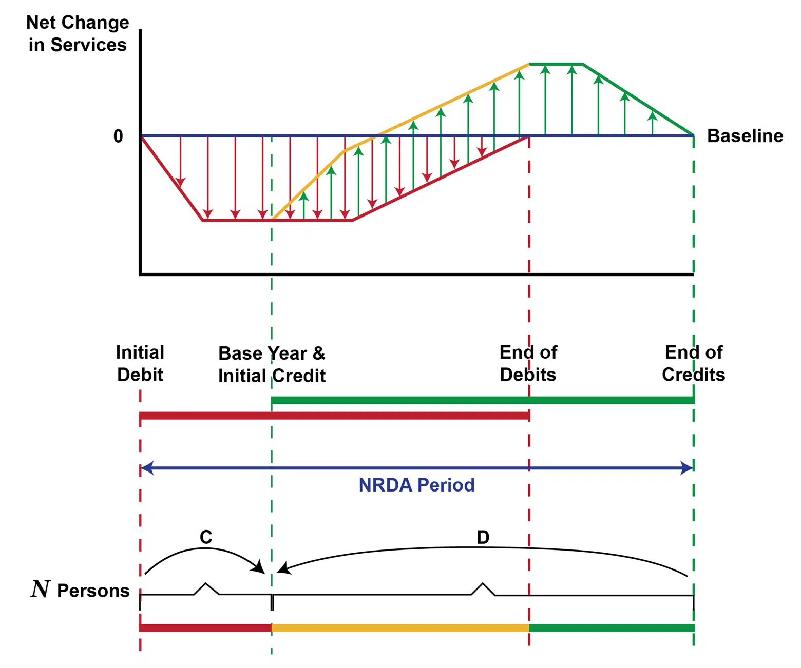
Figure 1. Discounting Long Lives

In Figure 1, debits are shown in red, credits are shown in green, and periods when both are operating are shown in yellow. The top portion of the diagram is the standard SEA graph of undiscounted services. The thinner red and green lines are service curves, and the associated arrows are quantified as changes from baseline. The net effects, to be discounted in the SEA, are shown as the thick red, yellow, and green lines. These quantified annual net debits and credits are projected down to the bottom portion of the figure, where discounting is applied. There are N identical affected persons, all born before debits begin and living until after credits end. Changes in well-being from debits and/or credits in each year occurring before the base year are compounded forward (shown as the curved arrow labeled C), and effects in years after the base year are discounted back (shown as the curved arrow labeled D).¹⁴ The scale of restoration does not depend on the choice of the base year. Figure 1 is what SEA spreadsheets implement. 

An alternative interpretation of the standard model, with more realistic demographics, is shown in Figure 2. This version reveals the ethical difficulties of the standard model. Individuals have finite lifespans that do not overlap. Four cohorts of individuals are shown, but in practice, there is a cohort for each year. 

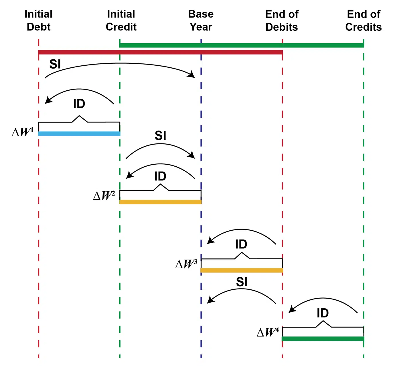
Figure 2. Discounting with Identical Cohorts

There are N identical individuals born into each cohort. Each person discounts the effects experienced within their lives to their birth date. Individuals’ discounting is depicted by arrows labeled ID. The effect of debits and/or credits on their lifetime well-being is denoted by ΔWᶦ for the iᵗʰ cohort.  

The Trustees scaling computation has three steps: (1) take the within-lifetime discounted effects for each person as given on a descriptive basis, (2) multiply it by the N persons born into each cohort, and (3) add this value across the cohorts, weighting the effects on each cohort’s well-being by a factor that compounds the amount forward from birthdates before 2025 and discounts back from birthdates to 2025. The weighting factors are depicted in Figure 2 as arrows labeled SI, a mnemonic for Trustee discounting using a rate of “social impatience”. The aggregation over the affected population in the third step of the computation is a normative (ethical) choice of a weight attached to each cohort based on when those persons are born.  

If the Trustees’ rate of social impatience in Figure 2 is the same as individual impatience in Figure 1, the two interpretations of standard SEA discounting are computationally equivalent.¹⁵ Therefore, we have demonstrated that standard SEA discounting involves birthdate discrimination. This is ethically equivalent to, say, determining the value of effects of injury on recreation for each person in a population in a single year and then summing that value across persons after applying a weight based on some attribute of that person, such as their height. Applying a weight to each cohort violates an “anonymity” principle in which individuals’ names, or other ethically irrelevant aspects of individuals, are not used in social decision-making.¹⁶ There is no economic rationale for the “extra” discounting undertaken in the SEA and on this basis, we assert that the standard approach to discounting embodying social impatience is unsound.  

If cohort discrimination is expunged from the step in which individual present values are aggregated, there is no need for a “base year”. Each person’s discounted lifetime value is calculated and simply added together to compute the change in public well-being across all cohorts.  

The Standard Discounting Model: Changing Populations 

Significant population change has and/or will occur over the time period of debits and credits in most NRDAs. This is a material consideration, especially in some state cases that seek recoveries in the distant past. The model of discounting exhibited in Figure 2 can be altered accordingly by multiplying by the different numbers of individuals in each cohort before summing over those cohorts.  

The Standard Discounting Model: Changing Baselines 

In this section, we set aside the impatience and population change issues addressed in prior sections; none of the conclusions here are altered by this assumption, and everything from the prior sections applies here with equal force. 

As noted, the 3% discount rate, based on BCA thinking, assumes monetization of effects. The “good” being traded across time in BCA can be thought of as aggregate consumption good (roughly GDP in which goods are aggregated by their market prices). Setting aside impatience and population changes, there is a discount rate in BCA because GDP generally has been growing over time. An investment today (1) reduces consumption when the public is relatively poor and an extra unit of consumption is relatively highly valued, then (2) increases consumption in the future when the public is relatively rich and an extra unit of consumption is of lower value. The ratio of these per-unit values in different periods defines the discount rate in BCA (absent impatience). The greater the rate of growth in GDP, the greater the rate of return investment must be to compensate for the falling value of the units of consumption it creates, implying a larger discount rate. This reasoning is the basis of discounting for monetized effects.  

In SEA, there is no monetization of service changes; rather, ecological services themselves are being traded over time. A discount rate may arise if the regional baseline level of services changes over time. It is this ecological discount rate (see Gollier 2013) that applies in SEA (Tomasi et al. 2024). Therefore, the 3% rate, taken from financial markets and manifestly not an ecological discount rate, does not apply in SEA. 

If baseline services are increasing over time, the same rationale for a discount rate as that in BCA applies to the ecological discount rate. A service loss in the past from a low baseline is highly impactful on well-being, while future restoration augments an already robust baseline and is less highly valued. The greater the percentage rate of growth in baseline services, the greater the discount rate. Conversely, if services are falling, the opposite effect holds, and the ecological discount rate is negative (absent impatience). Therefore, to the extent that baseline services are changing in different ways over the timespan of effects in a NRDA, the appropriate ecological discount rate varies as well.  

A Simple Example of Individualistic Discounting in SEA 

In this section, we provide an example that brings together the three influences on social value over time that we discussed separately above: individual impatience, a changing baseline, and population dynamics. 

Model Demographics 

While it is possible to develop a more elaborate demographic model with new cohorts of individuals born each year who have different lifespans, for simplicity, we use the model of Figure 2. Here, we slightly modify the example used in Tomasi et al. (2024) and assume 100% injury begins in 1900 and lasts until 2030. Additionally, restoration begins in 2030 and provides 100% services until 2140. The periods for individual’s lifespans are the dates of the decadal censuses (i.e., the cohort born in 1900 lives until 1910 and so on for other cohorts).¹⁷ For population numbers until 2020, we use the average U.S. population of the bracketing census counts. For example, for the 1900–1910 population, we use 84.2 million individuals, which is the average of the U.S. population of 76.2 million in 1900 and 92.2 million in 1910.¹⁸ For populations after 2020, we use projections from the Weldon Cooper Center for Public Service at the University of Virginia (UVA 2024) until 2050, after which we use a constant population. The time path of populations is depicted in Figure 3. As required by the standard SEA, we assume that individuals have identical preferences for services within and across cohorts. 

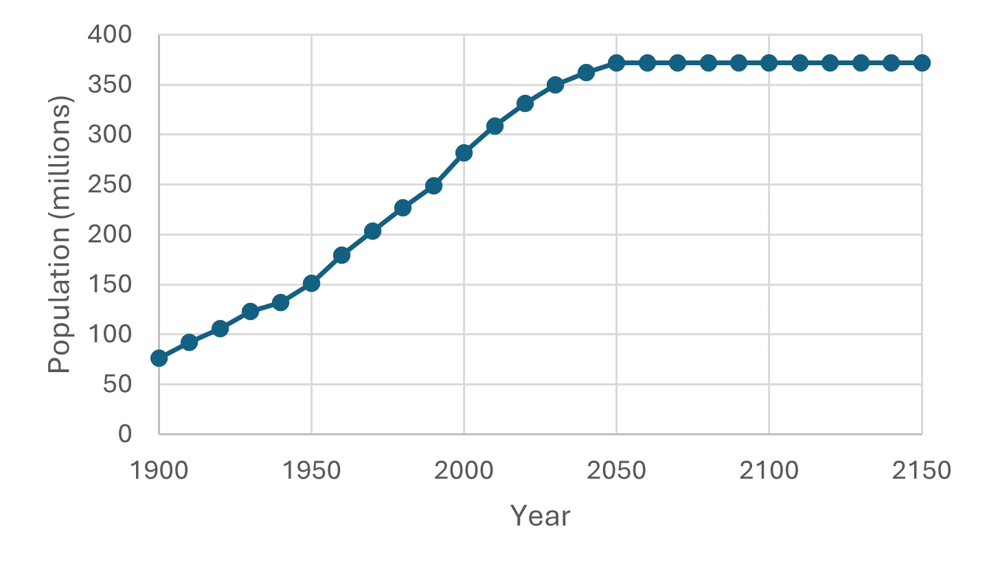
Figure 3. U.S. Population Over Time

Within each cohort, the discount rate is given by the equation d=δ+(g×γ), where δ is the rate of impatience individuals use to discount within their lifetimes, g is the positive or negative growth rate in baseline services over the decade, and 𝛾 is a parameter that governs how a given percentage change in baseline services gives rise to a percentage change in the incremental value of services.¹⁹  

For the individual rate of impatience, we use 𝛿=1.25% and discount service effects to the cohort’s birth year. Adopting the anonymity principle, we do not employ a social rate of impatience and aggregate effects on individuals as a simple sum.²⁰ Hence, there is no need for a “base year” for discounting.  

Our assumed baseline changes over the decadal periods and the associated discount rates for each decade are provided in Table 1.²¹ We assume the site is an urban waterway in an industrial area and that the NRDA issue is contaminated sediments addressed using HEA, with debits and credits denominated in discounted service acre years (DSAYs). 

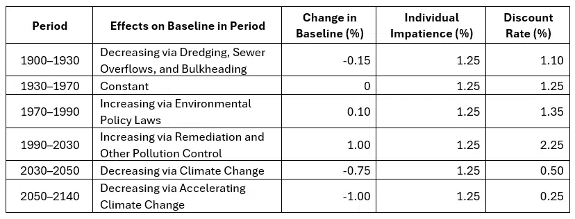
Table 1. Assumed Baseline Changes and Discount Rates

Regarding the effect of a changing baseline, we implement three versions of the model. In the first, we specify that 𝛾=0, which is consistent with Condition 2(b) above and some evidence from the literature on economic values of ecosystem services that finds very small values for 𝛾 (Tomasi et al. 2024). In this case, individual discounting is at the rate of impatience alone (1.25%). In the second version, we again specify that 𝛾=0 but use a discount rate of 3%. In the third version, we specify that 𝛾=1; in this case, a given percentage change in baseline services induces the same percentage increase in the value of a small change in services. Here, the discount rate is the sum of impatience (1.25%) and the percentage rate of change in baseline services in each period.²²  

Site characteristics and restoration costs are the same as in Tomasi et al. (2024)—i.e., it is a 100-acre site, and restoration costs $100,000 per acre. Table 2 summarizes the implications of discounting in various scenarios in this example.  

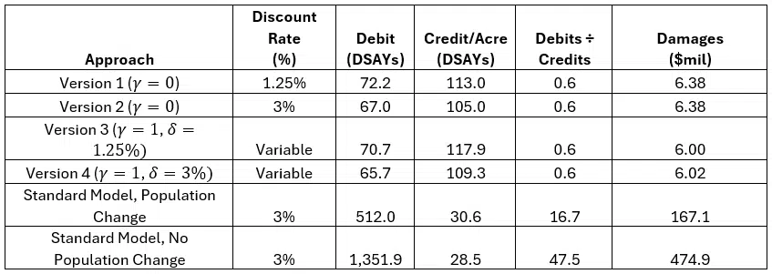
Table 2. Differing SEA Results Across Discounting Options

In this example, the most influential distinctions between the standard model and the approach adopted in this paper are the following (in decreasing order): (1) excising discrimination by birth year from the analysis, (2) accounting for population change, (3) adopting ecological discounting rather than financial discounting, and (4) the sensitivity of the value of a service change to the baseline from which it is measured (𝛾=0 or 𝛾=1). 

In our view, the first three distinctions should not be controversial. The value of 𝛾 for ecological resources is more of an open question, but it clearly is less important than the other three modifications of the standard model. The influence of the third distinction is due in part to the potentially modest percentage changes in baseline services assumed in our example. However, it is hard to see how this would become more important than the other issues unless future losses in services are catastrophic.  

The cohort discrimination occurring in the Trustee approach accounts for a staggering fraction of estimated damages in this example. Of the 1,351 DSAYs lost prior to restoration, only 114 of those are incurred by cohort members during their respective lifetimes. Thus, of the 1,237 DSAYs in the standard model with population change, 92% are from weighting individuals according to birthdate. Cohort discrimination alone reduces restoration benefits by 73%.  

Extensions 

The discounting model of the previous section is an advance on the standard model, but it has simple demographics. It is possible to generalize this approach to versions that are incrementally more general but computationally more intensive. These versions retain the basic structure of discounting within individuals’ lifetimes and simple summation across individuals without weighting.  

The first generalization is the introduction of nonuniform lifespans. Cohorts are identical, but individuals born into each cohort live to different ages. Incorporating this effect involves a simple adjustment that modifies the population size of each cohort to reflect the fraction of those born on a given date who live a given lifespan. Thus, if there are N persons born into a cohort at date t, and a fraction f(s) of them live to age s, then the average discounting of that cohort adds up, across lifespans, the discount factor from age s to date t using the rate of impatience.²³      

The next generalization allows the age class distribution and the population to change over time. Because the age class distribution is known accurately only via the decadal census, one can interpolate between the fractions at different ages for the intervening years.  

The final generalizations add uncertainty. One source of uncertainty is in lifetimes, which affects individual decision-making. In this formulation, the impetus for individual discounting is not necessarily pure impatience; rather, it is an uncertain time of death (Bommier 2006), or perhaps it is a combination of the two. The second source of uncertainty is about the future growth rate of regional baseline services. This issue has been much discussed in the literature on discounting in the BCA of climate change policies and the social cost of carbon; generally, more uncertain future rates of change in baseline services call for a lower discount rate, and because more distant futures are more uncertain, discount rates decline over time, all else remaining equal.   

Discussion 

We have shown that the standard discounting model in SEA is deeply flawed. First, the 3% discount rate, based on historical financial market returns, is incorrectly applied in an SEA setting, where ecological service units are estimated as opposed to monetary gains and losses. Second, fluctuations in impacted populations and baseline services are not incorporated into the standard SEA model. Third, and most importantly, the standard model applies an “extra” discounting effect that adjusts impacts on individual well-being according to individual birthdate. This final point clearly is ethically problematic and has no place in Trustee decision-making about how to protect public trust. 

Each distinction can cause significant differences in SEA estimates of debits and credits in its own right, and more so when applied together in the same model. To remedy these deficiencies, we propose a more realistic demographic model in which individuals have finite lifetimes. Those individuals exhibit impatience in their behavior, which is respected by Trustees. However, having accounted for individual impatience, there is no normative basis for adding social impatience.  

We also propose that scaling computations account for population changes over time when discounting in SEA, just as they do when monetizing debits and credits. There is no logical rationale for ignoring the fact that public values depend on how many individuals experience a change in services. 

Finally, we propose that the proper evolving baseline to define a discount rate applied to service changes is baseline services, not an evolving baseline of monetized goods (GDP).  

Our proposals result in a more appropriate discounting of debits and credits over time. In this paper, we have discussed the complex nature of these issues and provided an example that, while admittedly simplified, serves as a primer on how discounting in SEAs should be conducted. This paper also provides a new starting point for practitioners to estimate restoration scale in a defensible manner.  

References 

Bommier, A. 2006. Uncertain Lifetime and Intertemporal Choice: Risk Aversion as a Rationale for Time Discounting. International Economic Review 47:1223–1246.  

Desvousges, W., N. Gard, H. Michael, and A. Chance. 2018. Habitat and resource equivalency analysis: A critical assessment. Ecological Economics 143:74–89. doi: 10.1016/j.ecolecon.2017.07.003. 

Dunford, R.W. 2018. The discount rate for assessing intragenerational natural resource damages. Journal of Natural Resources Policy Research 8:89–109. 

Dunford, R.W., T.C. Ginn, and W.H. Desvousges. 2004. The use of habitat equivalency analysis in natural resource damage assessments. Ecological Economics 48(1):49–70.  

Flores, N.E., and J. Thacher. 2002. Money, who needs it? Natural resource damage assessment. Contemporary Economic Policy 20(2):171–8. doi: 10.1093/cep/20.2.171. 

Freeman III, A.M., J.A. Herriges, and C.L. Kling. 2014. The Measurement of Environmental and Resource Values: Theory and Methods. Third edition. RFF Press, New York, NY. doi: 10.4324/9781315780917.  

Gollier, C. 2010. Ecological Discounting. Journal of Economic Theory 145:812–839. 

Gollier, C. 2013. Pricing the Planet’s Future: The Economics of Discounting in an Uncertain World. Princeton University Press, Princeton, NJ. 

Gollier, C., and J. Hammitt. 2014. The long-run discount rate controversy. Annual Review of Resource Economics 6:8.1–8.23. 

Hoel, M., and T. Sterner. 2007. Discounting and relative prices. Climatic Change 84:265–280. doi: 10.1007/s10584-007-9255-2. 

Horsch, E., D. Phaneuf, C. Gihuere, J. Murray, C. Duff, and C. Kroninger. 2022. Discounting in Natural Resource Damage Assessment. Journal of Benefit-Cost Analysis 14(1):1–21. doi: 10.1017/bca.2022.24. 

Jones, C., and K. Pease. 1997. Restoration-Based Compensation Measures in Natural Resource Liability Statutes. Contemporary Economic Policy 15(4):111–122. 

Malinvaud, E. 1953. Capital Accumulation and Efficient Allocation of Resources. Econometrica 21:233–268. 

Mazzotta, M., J. Opaluch, and T. Grigalunas. 1994. Natural resource damage assessment: The role of restoration. Natural Resources Journal 34:153–78. 

McFadden, D., and K. Train (eds). 2017. Contingent Valuation of Environmental Goods: A Comprehensive Critique. Edward Elgar Publishers, Northampton, MA. 

Millner, A., and G. Heal. 2023. Choosing the Future: Markets, Ethics, and Rapprochement in Social Discounting. Journal of Economic Literature 61:1037–1087. 

NOAA. 1999. Discounting and the Treatment of Uncertainty in Natural Resource Damage Assessment. Technical Paper 99-1. National Atmospheric and Oceanic Administration, Damage Assessment Center, Resource Valuation Branch, Silver Spring, MD. 

OMB. 2023. Guidelines and Discount Rates in Benefit-Cost Analysis of Federal Programs. Circular A-94. Office of Management and Budget, Washington, DC. 

Tomasi, T., R.W. Cooper, and D. Anning. 2024. On the discount rate in environmental damage cases. Environmental Claims Journal 37(1):1–30.  

doi: 10.1080/10406026.2024.2440574.  

Unsworth, R., and R. Bishop. 1994. Assessing natural resource damages using environmental annuities. Ecological Economics 11(1):35–41. doi: 10.1016/09218009(94)90048-5. 

UVA. 2024. National Population Projections. https://www.coopercenter.org/national-population-projections. University of Virginia, Weldon Cooper Center for Public Service, Charlottesville, VA.