Considering Environmental Justice in Natural Resource Damage Assessment: Injury to Ecological Resources

Abstract

Determining the scale of restoration needed to compensate the public for injuries to natural resources is central to estimating natural resource damages for unpermitted releases of contamination. This paper discusses the inclusion of environmental justice in formal restoration scaling models for injury to the ecological services of resources. These are services that people do not use directly; current practice almost exclusively employs service equivalency scaling models that do not use economic values. Heretofore, service equivalency models have assumed that people have the same preferences for different services. If preferences are not the same, the chosen restoration will leave some persons overcompensated and others undercompensated. In this case, a method for aggregating over people is needed to determine when restoration compensates the public as a whole. An aggregation method that does not rely on economic values has yet to be specified. Therefore, service equivalency methods currently have no rational foundation in an economy with heterogeneous preferences for nature’s services. Incorporating environmental justice in natural resource damage assessment requires an aggregation procedure that recognizes ethically relevant differences among affected persons. Because there is no method whatsoever to aggregate over heterogeneous people, there clearly does not exist one that recognizes environmental justice. This paper fills these two gaps; it provides a way to aggregate effects over people without using economic values, and the method proposed allows for environmental justice to be incorporated into scaling by favoring restoration that effectuates a transfer from the resource rich to the resource poor. The approach relies on information about individuals’ preferences that allows them to be aggregated, but does not require economic valuation of nature’s services.

¹I wish to acknowledge helpful comments from David Anning, Heath Byrd, and George Parsons, while absolving them of remaining errors and opacities.

Introduction

Natural resource damages (NRDs) associated with releases of contaminants to the environment equal the cost of resource restoration projects, the benefits of which offset injuries to natural resources. The key issue for the magnitude of damages is identifying the type and amount of restoration needed to redress the harm; this is called restoration scaling. In this paper, I outline an approach to scaling that builds environmental justice into the computations using an index of social welfare that includes considerations of equity. I call this “social valueto social value” (SVtoSV) scaling. I focus here on impacts to ecological service losses that are not the object of direct human uses.

Including environmental justice in scaling is relatively straightforward when economic values for the services provided have been estimated. In a companion paper, I discuss including environmental justice in (SVtoSV) restoration scaling for recreation, where valuation is standard practice (Tomasi 2021). There it is shown how the social welfare index that considers equity can be constructed from individual values for services. The methods developed in that paper would apply as well to non-use services for which reliable economic values have been obtained. However, valuation of non-use services is controversial and rarely used in natural resource damage assessments (NRDAs) for non-use services.² Instead, NRDAs for such services typically employ service equivalency scaling methods, such as resource equivalency analysis (REA) and habitat equivalent analysis (HEA), which do not employ economic values.³

Generally, a habitat or resource will provide a number of different services that are injured and restored to varying degrees. A compensatory restoration project will provide one bundle of these services to the public. If people have different preferences over services, they may not agree about the amount of restoration that will compensate them for the injury, and any given restoration project will leave some undercompensated and others overcompensated. To date, absent economic values for services, NRDA practitioners have not identified any way to aggregate over a population with heterogeneous preferences for natural resource services to determine whether, on net, compensation of the public as a whole has been achieved. Therefore, NRDA practitioners must assume that people agree on restoration scale by assuming they have identical preferences for the various services natural resources provide.

Assessing environmental justice fundamentally involves evaluation of outcomes across individuals that differ in some ethically relevant way that decision makers may wish to consider in evaluating restoration alternatives. Without a way to aggregate across people at all in REA and HEA, there obviously is no way to aggregate across them to reflect concerns for environmental justice.

REA and HEA operate with minimal information about peoples’ preferences. Nothing more is known about them than that more of any one service is preferred to less. If this is definitional of the methods, then we are at an impasse and there seemingly is no way around the assumption that people have identical preferences. In this paper, I provide two key results that allow the applicability of REA and HEA to be expanded. First, I show that in REA, people can have divergent preferences for services, yet agree on the amount of restoration needed to compensate for injury. This requires a special form of preferences, but one less restrictive than that they are identical. No additional information is needed to implement the REA beyond a comfort level that the weaker assumption is likely to hold in most cases. This amount of information does not allow consideration of environmental justice, but it does provide a firmer foundation for applying REA when we believe the public holds different preferences for services.

²I lump indirect-use services in with non-use services in this paper, as REA and HEA include both. An example of indirect use is when effects on wetlands alter catch rates for sport-caught fish and thereby the value of recreational angling. Some difficulties of valuing nonuse services of natural resources are described in McFadden and Train (2017).
³Wakefield et al. (2022) provide a thorough overview of HEA and REA methods.

The aforementioned result does not apply to HEA. The second result is a way to aggregate preferences over people with disparate preferences in HEA (or in REA when the restriction on preferences does not apply) by adding information about peoples’ preferences, but without resorting to economic valuation. The aggregation procedure has the additional property that it incorporates environmental justice.

Restoration Scaling

My discussion is based on a stylized representation of an NRDA case that allows a simpler presentation of the basic ideas. There are two time periods, two ecological services provided at levels 𝑄₁ and 𝑄₂, and two people named a and b. I let 𝑄 = (𝑄₁,𝑄₂) be a “service bundle.” The sequence of events is as follows:

• In the beginning of the first period, a spill of oil or release of a hazardous substance reduces ecological services. Baseline services, denoted by 𝑄^B, are reduced to 𝑄^𝐼 by an amount of injury ∆^𝐼.Injury is constant until it is remediated.
• In response to the event, the habitat is cleaned up and the area restored to its prior condition. This takes place at the end of the first time period and instantaneously provides service levels that are equivalent to services under baseline conditions.
• The NRDA takes no time to complete. The process identifies compensatory restoration for the interim loss of recreation services from the time of the release to when the recreation site is back to baseline conditions.
• The restoration project is implemented in the beginning of the second time period, provides benefits instantaneously that are constant for one period, and then evaporates.
• Restoration increases services by an amount ∆^R to a restored level of services 𝑄^R. Services are at constant level 𝑄^R until the end of the second time period and then revert to baseline instantaneously.
• The discount rate is zero.

These simplifying assumptions allow me to concentrate on core issues of environmental justice; relaxing them alters the details of implementation but not the basic ideas I address. I do make the substantive simplifying assumption that people are identical in all regards except for their preferences for natural resource services, or equivalently for restoration scaling, that these other potential differences are not considered in NRDA. If there
are other dimensions of inequality, for example, in incomes, health status, or education, these are not built into HEA or REA scaling computations.

The problem faced by the natural resource trustees (Trustees), acting on behalf of the public, is to choose one restoration project from among the feasible alternatives; making this choice is called restoration scaling. A scaling method is a rule for ranking restoration projects. A project is a combination of location, design, and size. A scaling rule determines, for any two projects 𝑥 and 𝑦, whether the Trustees prefer 𝑥 to 𝑦, prefer 𝑦 to 𝑥, or are indifferent between them.

Project choice reflects several evaluative criteria for judging restoration. These criteria serve as axioms for scaling rules. For my purposes, the primary criteria are

In HEA and REA, the N is a technical requirement; restoration projects must provide services that would have the same per-unit values as those injured (Dunford et al. 2004). For example, if waterfowl are killed by an oil spill, restoration would be of waterfowl, perhaps not all the same species, but those that have similar ecological functions, for example in the same feeding guild. CE rules out unnecessarily large projects.⁴

As stated, PC is not very useful; some operational notion of public compensation is required. What is needed is an index of aggregate well-being based on the levels of services provided. This is true for any scaling method. Let 𝑈^𝑖(𝑄) be a numerical index of the level of well-being attained by person 𝑖 when provided the service bundle 𝑄. A social welfare function (SWF) specifies overall public well-being as a function of individual levels of well-being.⁵ The SWF is written as

𝑊(𝑄) = 𝑊[𝑈^𝑎(𝑄),𝑈^𝑏(𝑄)].

The SWF is consequentialist in that it depends ultimately on the services provided, and welfarist in that it depends on each individual’s evaluation of those consequences through the well-being functions 𝑈^𝑖(𝑄). The compensation axiom can be restated as follows.

⁴Other criteria and potential interplay among them are considered in the companion paper on recreation (Tomasi 2021).
⁵This is a slight abuse of terminology; there is at this point no requirement that this is a real valued function; it represents a social ranking of outcomes. Sen (2017, Chapter 3) provides a discussion.

A scaling model is a particular way to specify the welfare index. For recreation, where economic values are used without (much) controversy, the traditional welfare index is the difference in the simple (unweighted) sum over affected persons of the economic value each attaches to restoration and to injury. Economic values provide a common measuring rod for preferences that allows their aggregation as described in Tomasi (2021). With HEA and REA that do not use values, there is no direct way to compare preferences for service bundles across people in a way that they can be aggregated into an overall index. This paper forwards a method that accomplishes this task.

The social welfare index 𝑊 can be specified to include environmental justice by giving priority to those who would otherwise be relatively disadvantaged in terms of natural resource services. Thus, another axiom could be added to reflect the inclusion of environmental justice in scaling.

One commonly used approach to implementing EJ is to specify an SWF that increases when there is a balanced transfer of services (leaving the mean unchanged) from a relatively resource-rich person to a relatively resource-poor one, with no changes for anyone else.⁶

My approach is to reformulate HEA and REA to accommodate both Axiom 1-W and Axiom 4. Before doing that, I describe HEA and REA as traditionally applied.

1. Quantify the injury as the reduction in services provided by natural resources relative to what services would be at baseline. In my simple model, this is ∆^𝐼= 𝑄^𝐵 − 𝑄^𝐼.
2. Quantify the benefits of a compensatory restoration project that increases the injured services above what they would otherwise be at baseline. This is ∆^𝑅= 𝑄^𝑅 − 𝑄^𝐵.
3. Adjust the size of the project such that its service benefits equal the quantified injury. This requires that ∆^𝑅= ∆^𝐼.

HEA and REA require that there is a single measure of services. Because natural resources typically provide many services, they must be aggregated into a composite service index. Further, the composite service indexmust be constructed in the same way for both injury and restoration benefits. REA and HEA differ in how this aggregation is accomplished.\

⁶See Cowell (2016) for an introduction to inequality measures. Chakravarty (2018) provides the multi-dimensional case. Fleurbaey and Maniquet (2011) discuss a number of different versions of the transfer concept.

REA is applied to a single resource (such as a population of birds or volume of water), and it is assumed that each service is provided in direct proportion to the amount of the resource. Thus, the amount of resource is its own service aggregator and individual services need not be specified or measured. In contrast, HEA is applied to a unit of habitat that provides many different services. A composite service index is constructed as a weighted sum of the individual services, with weights determined by the Trustees. If scaling is to identify projects that compensate the public based on a consequentialist/welfarist approach, the composite index should reflect how individuals view the different services and weight them according to how those services affect their own well-being. That is, the weights should reflect individual preferences for the various services and their relative contribution to individual well-being.

The necessity of service weights creates a difficulty in applying HEA. Service weights should reflect individual preferences, but preferences are not measured when using HEA or REA. In practice, weights are assigned by practitioners acting without the benefit of direct and transparent information about the public. This opens the door to a degree of arbitrariness in using HEA in the NRDA process (Baker et al. 2020).

However, the difficulty of service weighting in HEA goes deeper. The services addressed by REA and HEA typically are public goods, which means that individuals do not choose how much service to enjoy.⁷ If individuals’ preferences for services differ, then any one project potentially will leave some persons overcompensated (“winners”) and others undercompensated (“losers”). In an early paper developing the economic foundations of HEA, Jones and Pease (1997) suggested that analysts apply potential compensation tests. In this approach, a restoration project is deemed to have compensated the public if the winners could (hypothetically) transfer enough money to the losers to leave them indifferent to their circumstances at baseline, and the winners could remain compensated after the transfer. This approach to determining whether the PC Axiom is satisfied is called the Kaldor-Hicks compensation test. This Kaldor-Hicks approach is applied in the traditional scaling of restoration for recreation resources in NRDA and is discussed in a companion paper (Tomasi 2021). There are two problems with such compensation tests.

The first problem is that the compensation is not actually carried out, so that losers remain losers and winners remain winners. Ethical judgments about who should win and who should lose are not part of the assessment. Thus, scaling based on compensation tests does not consider equity. 8 The second and more basic problem is that money, which is used in the hypothetical transfers, is not part of NRDA (as scaling is separable). Compensation in NRDA is required by law to be provided in-kind via restoration projects. Further, the whole point of HEA and REA is to avoid such monetary values. Thus, there seems to be no way to implement the Kaldor-Hicks test (Flores and Thatcher 2002).

⁷Services can also be local public goods, which provide services equally to all in a confined location, with different locations providing different bundles of services. I ignore this and assume that the nexus criterion locates restoration where it provides services equally to the same individuals as those injured.
⁸To clarify, if individual economic values for services exhibit an aversion to variation in personal enjoyment of services, then a simple summation as in the Kaldor-Hicks will reflect this aversion. However, this may not adequately represent social aversion to inequality across people. This is discussed further in Tomasi (2021).

On this basis alone, REA and HEA rest on shaky ground. Because compensation tests cannot be implemented, there is no basis for a claim that a given project is satisfactory to the public. The Trustees can assert only that they have compensated a fictitious person. It is easy to develop an example in which this can lead to the entire public, except one, consisting of losers. The idea that compensation is accomplished “on average” is generally incorrect, and a justification founded on potential compensation is not applicable.

Further, even if the potential compensation test could be in fact be implemented, given that no compensation is actually paid, the outcome is likely to be unfair and inconsistent with considerations of environmental justice.

The approach offered in this paper replaces the potential compensation test with a social welfare approach whereby the well-being of persons affected by injury and restoration is explicitly aggregated. This approach can address the first problem with the compensation axiom and therefore is an important advance irrespective of any consideration of environmental justice.

Economics of REA and HEA

Individual Preferences for Services

To say that a restoration project compensates the public requires some idea of what the public prefers in terms
of services. I assume that each affected person has preferences over bundles of services given by an ordering
relation 𝑅𝑖, which ranks alternative bundles. The relation 𝑄𝑅^𝑖𝑄′ is read “person 𝑖 judges bundle 𝑄 to be at least as good for him or her as bundle 𝑄′.” Strict preference is written 𝑄𝑃^𝑖𝑄′ and indifference is written 𝑄𝐼^𝑖𝑄′.⁹

I assume that the preference rankings are rational, which imposes two requirements. First, persons can rank any two bundles: either 𝑄𝑅^𝑖𝑄′ or 𝑄′𝑅^𝑖𝑄 or both. Second, preferences are such that, if 𝑄𝑅^𝑖𝑄′ and 𝑄′𝑅^𝑖𝑄′′, then 𝑄𝑅^𝑖𝑄′′ (this is called transitivity of preferences).

If preferences are rational, then given a set of possible restoration projects, each person can identify a project that is preferred or indifferent over any other in the set.10 I add to rationality two additional postulates. First, more services do not make persons worse off, and strictly more services make them better off. Second, preferences are convex; if 𝑄𝐼^𝑖𝑄′, then any weighted average of them is at least as good as either of them. Preferences are strictly convex if the weighted average is strictly preferred when it is not equal to either 𝑄 or 𝑄′.¹¹

⁹Strict preference occurs when 𝑄𝑅𝑖𝑄′ holds and 𝑄′𝑅𝑖𝑄 does not; indifference occurs when both 𝑄𝑅𝑖𝑄′ and 𝑄′𝑅𝑖𝑄 hold.
¹⁰Having rational preferences means that for each set of possible service bundles 𝑆 there is a subset of them 𝐶(𝑆|𝑅) such that there is no bundle in 𝑆 outside of 𝐶(𝑆|𝑅) that is preferred to any bundle in it. 𝐶(𝑆|𝑅) is called a choice set for the set 𝑆 evaluated via preferences 𝑅. That a choice set exists does not mean that agents actually choose from it when given the chance. An additional assumption of rational choice says that agents actually make choices from feasible choice sets. Observed choices can reveal preferences only if agents are rational choosers and are informed about the possibilities, and so involve their beliefs about what is available and feasible (see Hausman 2012).

With two services and these assumptions on preferences, preferences for each person can be represented graphically by indifference curves, which are all combinations of service bundles that an individual judges to be indifferent to one another. Two strictly convex indifference curves are shown in Figure 1.¹²

In Figure 1, the two services are on the axes. Start with the baseline bundle 𝑄^𝐵. The indifference curve through this bundle is a plot of all the bundles that the individual ranks the same as the baseline bundle according to

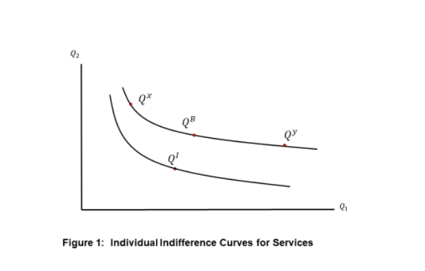
their preferences. The indifference curve through 𝑄^𝐼 is similarly defined relative to the service bundle with the injury. Compared to 𝑄^𝐼, bundle 𝑄^𝐵 has more of both services; hence, baseline is preferred to injury by the monotonicity postulate. Any bundle strictly “northeast” of a bundle 𝑄^𝐼 is preferred; as such, 𝑄^𝑦 surely is strictly preferred to 𝑄^𝐼. But being northeast is not necessary for strict preference. Any bundle on the indifference curve through 𝑄^𝐵 is preferred to any point on the indifference curve through 𝑄^𝐼 by the postulate of transitivity in the definition of rational preferences. Therefore, 𝑄^𝑥 is preferred to 𝑄^𝐼 even though it has less of 𝑄₁, as it has enough more of 𝑄₂ to make up for this.

¹¹Preferences are strictly monotonic: if 𝑄 ≥ 𝑄′, then 𝑄𝑅^𝑖𝑄′ and if 𝑄 > 𝑄′, then 𝑄𝑃^𝑖𝑄′. Convexity of preferences means that if 𝑄𝑅^𝑖𝑄′ and 𝑄′′ = 𝜃𝑄 + (1 − 𝜃)𝑄′, then 𝑄′′𝑅^𝑖𝑄 for all 0 ≤ 𝜃 ≤ 1. Strict convexity means that 𝑄′′𝑃^𝑖𝑄 for all 0 < 𝜃 < 1
¹²I also add a technical condition that preferences are continuous, which means that there are no gaps in the indifference curves with a very small change in services leading to a jump in preference.

I equate the level of individual well-being attained by a person with the extent to which their preferences are satisfied. With this assumption, an indifference curve establishes a level of well-being, or personal welfare. There is ethical content to this assumption that has been much discussed by economists and philosophers (see, for example, Hausman et al. 2017 for an introduction and Hausman 2012 for an in-depth discussion).

Scaling with Indifference Curves

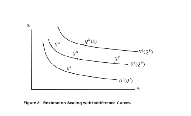
Figure 2 adds another indifference curve above the baseline one, and numbers the curves with a utility function. A utility function is a numerical index that represents the preference ranking, with higher numbers assigned to higher indifference curves. A utility function is an aggregator of the two services into a single numerical index according to an individual’s preferences.

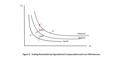
Recall that the injury moves the person from 𝑄^𝐵 to 𝑄^𝐼 for one period, and restoration project 𝑥 moves the person from 𝑄^𝐵 to 𝑄^𝑅(𝑥) for one period. Therefore, project 𝑥 compensates this person if the difference between the levels of well-being attained at 𝑄^𝐵 and 𝑄^𝐼 is at least as great as the distance between 𝑄^𝐵 and 𝑄^𝑅. This begs the question: how is distance measured? Pick 𝑄₂ as a “numeraire.” The vertical distance downward from the baseline service bundle to the indifference curve associated with the injured services is the willingnessto-pay (WTP) of person i (in units of 𝑄₂) to avoid the spill and remain at 𝑄^𝐵. If an amount ∆₂^𝑅 of 𝑄₂ is added to the baseline bundle, this is person 𝑖’s willingness-to-accept (WTA) compensation to forego the bundle (𝑄₁,𝑄₂ + ∆₂^𝑅) and remain at 𝑄^𝐵. This is the value (in units of 𝑄₂) of any restoration project that lies on the indifferent curve through (𝑄₁,𝑄₂ + ∆₂^𝑅). Restoration is scaled in the view of person i when WTP equals WTA at bundle A in Figure 3. The bundle at A is one scaled project, but all the bundles on the indifference curve labeled “Restored” also exactly compensate person i. A restoration project providing the bundle 𝑄^𝑅 would be judged by person i to be equally as good.

Service Equivalency Analysis

Both HEA and REA proceed from three assumptions. The first is that the two services are aggregated into single composite indicator 𝑄̂. The second is that changes in services from baseline due to both injury and restoration (∆^𝐼 and ∆^𝑅) pertain to the same composite service. With these two assumptions,13 the changes in utility can be rewritten as:

𝑚^𝑖∆^𝐼 + 𝐾^𝐼 = 𝑚^𝑖∆^𝑅 + 𝐾^𝑅.

In Equation 2, the term 𝑚^𝑖 is a constant and the terms 𝐾^𝑗 are “remainder” terms that depend on the amount of injury and restoration as well as the shape of the utility function 𝑈^𝑖. Importantly, the term 𝑚𝑖 is the incremental utility from a small increase in the level of the composite service from the baseline level of services. The third assumption is that the sizes of the injury and restoration effects are “small enough.” In this case,

¹³A technical condition, also required, is that the utility functions are differentiable.

no matter what the shape of the utility function, the remainder terms are small and we have the approximate result:

𝑚^𝑖∆^𝐼≈ 𝑚^𝑖∆^𝑅.

Because the term 𝑚^𝑖 is a constant (by virtue of the first two assumptions), it cancels out of Equation 3 and we are left with:

𝑆𝑒𝑟𝑣𝑖𝑐𝑒 𝐸𝑞𝑢𝑖𝑣𝑎𝑙𝑒𝑛𝑐𝑦: ∆^𝐼= ∆^𝑅

If the assumptions hold, satisfying Equation 4 leads to approximate compensation of individual 𝑖.¹⁴

Resource Equivalency Analysis

REA and HEA are distinguished by the way that they aggregate the two services into a composite service indicator. REA assumes that all services are supplied in direct proportion to the amount of the resource. Thus, if 𝐴 is the amount of resource, REA assumes that 𝑄1 = 𝜔1𝐴 and 𝑄2 = 𝜔2𝐴. Service provision in REA is shown in Figure 4.

In Figure 4, the two services are produced along a ray from the origin with a slope equal to 𝜔2⁄𝜔1. The axes

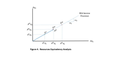
¹⁴If the utility function is highly curved in service levels (the marginal utility changes dramatically as the base level of services varies), then the changes must be quite small; if the utility function is linear (marginal utility is the same for all levels of services), then the change can be of any size.
are the amount of service produced per amount of the resource. The total amount of resource is given by the distance along the ray from the origin equal to the amount of the resource. Hence, in Figure 4, the baseline amount of resource is given by the length of the arrow from the origin to the service bundle 𝑄^𝐵. Suppose the amount of resource decreases by ∆^𝐼 from 𝐴^𝐵 to 𝐴^𝐼 for one period; services would fall from 𝑄^𝐵 to 𝑄^𝐼. Scaled restoration increases the resource by the amount ∆^𝑅 from 𝐴^𝐵 to 𝐴^𝑅 for one period (recall the discount rate is zero) and services increase from 𝑄^𝐵 to 𝑄^𝑅. REA implements Equation 4 by equating the distances along the REA service ray from 𝑄^𝐵 to 𝑄^𝐵 and from 𝑄^𝐵 to 𝑄^𝑅.

A basic question is whether REA implements individual compensation as defined by Equation 4. I answer this question via the scaling thought experiment depicted in Figure 2. In Figures 5a and 5b, I superimpose Figures 2 and 3. In Figures 5a and 5b, person 𝑖 is fully compensated by restoration of the resource along the REA ray sufficient to provide service bundle 𝑄^{𝑅−𝑉𝑡𝑉}. REA has restoration increases to the resource above 𝑄^𝐵 by an amount ∆^𝐼 that equals the distance along the REA ray equal to ∆^𝐼. REA restoration therefore provides bundle 𝑄^{𝑅−𝑅𝐸𝐴}. In Figure 5a, we have 𝑄^{𝑅−𝑉𝑡𝑉} greater than 𝑄^{𝑅−𝑅𝐸𝐴}. In Figure 5b, 𝑄^{𝑅−𝑉𝑡𝑉} is less than 𝑄^{𝑅−𝑅𝐸𝐴}. Thus, we see that REA can over- or underestimate NRDs.


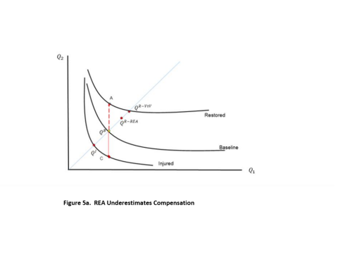
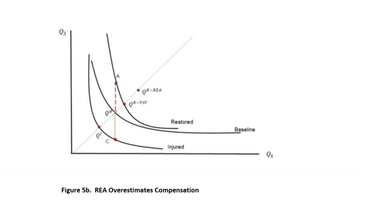
The reason for the potential mismatch between individual compensation and REA compensation is that the slopes of the indifference curves through the baseline, injured, and restored bundles diverge significantly. If the slopes of the indifference curves were the same through these points, then REA does implement exact individual compensation. Moreover, in this case, the amount of restoration would not depend on whether we chose 𝑄₁ or 𝑄₂ as our unit of value for individual scaling, while with preferences as drawn in Figures 5a and 5b, it would matter. Preferences that have indifference curves with the same slope along all rays from the origin are called homothetic. It can be proven algebraically that, with homothetic preferences, restoration using either value-to-value scaling (in units of either service) or REA are the same.

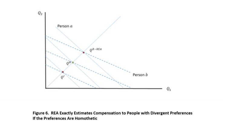
Moreover, this is true for any two persons even if they have different preferences. In Figure 6, I show indifference curves for two people: 𝑎 and 𝑏. These are drawn as parallel straight lines and therefore are homothetic. The slopes of their indifference curves diverge from one another, and so they do not have the same 𝑊𝑇𝑃 and 𝑊𝑇𝐴 for injury and restoration. However, they agree on the amount of restoration. This can be proven by a simple geometric argument by applying the analysis in Figure 4 to the curves in Figure 6. The proof can be extended to preferences that are homothetic and strictly convex so indifference curves are not straight lines.

Based on the above, statements in previous literature on HEA that people must have identical preferences in service equivalency scaling (e.g., Dunford et al. 2004; Desvousges et al. 2018; Flores and Thatcher 2002) is not true with REA. I can go a little further and assert that preferences do not have to be homothetic everywhere—they just have to have this property in the range of variation of injury and restoration, and so can be locally homothetic. Finally, if the amount of injury and restoration is small enough, preferences must be approximately locally homothetic because there is just not enough space for indifference curves to diverge significantly.¹⁵

Habitat Equivalency Analysis

The foregoing discussion does not apply to HEAs in which services can be provided in any combination. Of course, if the mix of services in an HEA is the same in both the injured and restored states as at baseline, then HEA effectively becomes an REA with acres of habitat as the amount of resource. In this case, all of the results

¹⁵This requires utility functions to be continuous.

described in the previous section apply. In the more general case of a true HEA (called HEA henceforth), the composite service index is formed as:

𝑄̂ = 𝜔₁𝑄₁ + 𝜔₂𝑄₂

where the 𝜔_𝑗 is service weight. If the HEA is to reflect a welfarist analysis, the weights should relate to public preferences for services. In this case, Equation 5 would be re-specified as:

𝑄̂_𝑖 = 𝑚₂^{𝑖𝑄₁ + 𝑚₂𝑖𝑄₂}

Each individual forms their own view of the composite index. In Equation 6, the weights are marginal utilities, reflecting the relative contribution of each service to preference satisfaction. Therefore, an HEA consistent with public preferences would set 𝜔𝑗 = 𝑚𝑟 where person 𝑟 is some “representative” individual. This representative individual exists if all members of the public have identical and homothetic preferences. This is stronger than for REA, where preferences need to be homothetic, but not identical.

HEA founders methodologically because different persons form different composite service bundles, whence there is no single individual who represents the public.

Preference Aggregation in HEA Models: REA-Equivalent Utility

What is needed is a way to make preferences comparable across people and to measure them on a common scale so they can be compared. Figure 7 shows the essential difficulty. Similar to Figure 6, it depicts two people: 𝑎 with solid indifference curves and 𝑏 with dashed ones. The Trustees are evaluating service outcomes associated with two projects: 𝑥 and 𝑦. As shown, person 𝑎 prefers 𝑥 to 𝑦, while person 𝑏 prefers 𝑦 to 𝑥.

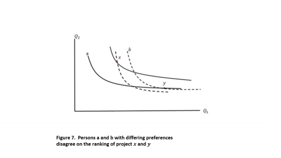
Given that these indifference curves provide only relative rankings, it is not possible to tell which person is better off than the other. It is not meaningful to ask whether the amount that person 𝑎 is better off than 𝑏 with project 𝑥 is more than the amount that person 𝑏 is better off than 𝑎 with project 𝑦. That is, there is no basis on which the trustees can rank the two projects and determining whether the PC axiom is satisfied is not possible. The essential point made by Flores and Thatcher (2002) is that you need value information and the KaldorHicks potential compensation criterion to make such a determination, and hence HEA is not a viable scaling method.

Figure 8 shows a way to address this conundrum. It adds an REA service curve, with the services per acre provided in fixed proportions equal to those exhibited in the baseline habitat. This is a hypothetical REA—it does not have to be feasible to actually provide services in fixed proportions over the range of injury and potential restoration. I will call this the “REA habitat.”

The proposed approach for utility measurement for preference aggregation asks, given an REA habitat with

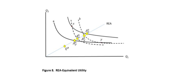
per-acre services fixed in the same proportions as in the HEA baseline, how much acreage of this habitat provides total services levels that are indifferent to those provided by the alterative HEA outcomes? The answer to this question is given by the points labeled 𝐴_𝑗^𝑖 (for 𝑖 = 𝑎, 𝑏 and 𝑗 = 𝑥, 𝑦). Starting with project 𝑥, person 𝑎 is indifferent between the services generated by that project and the point 𝐴𝑥𝑎 where 𝑎’s indifference curve crosses the REA habitat service curve. Thus, the distance 0𝐴_𝑥^𝑎 is the acreage of habitat that person 𝑎 ranks as indifferent to the HEA outcome [𝑄₁(𝑥),𝑄₂(𝑥)]. Similarly, person 𝑏 is indifferent between the outcomes under project 𝑥 and the point 𝐴_𝑥^𝑏. Because 𝐴_𝑥^𝑏 < 𝐴_𝑥^𝑎, person 𝑏 is worse off under project 𝑥. Turning to project 𝑦, the relevant points are 𝐴_𝑦^𝑎 and 𝐴_𝑦^𝑏, with their respective REA habitat acreages.

The numbers 𝐴_𝑗^𝑖 label the indifference curves and so provide a utility function for each person.¹⁶ I call this “REAequivalent utility.”¹⁷ Moreover, the distances from the origin to 𝐴_𝑗^𝑖 are acreages. Thus, differences between them are meaningful, and comparisons of these distances across people are meaningful as well.¹⁸ Further, the measures are scale-invariant; changing from acres to square meters does not alter measurement of REAequivalent utility.

Social-Value-to-Social-Value Scaling with REA-Equivalent Utility

What remains is to define an aggregation rule for REA-equivalent utilities. Any method that does this provides a reasoned basis for conducting an HEA or REA to identify restoration that compensates a public with heterogeneous preferences for services. This solves the dilemma identified by Flores and Thatcher (2002) without resorting to monetization of services and potential compensation tests. Furthermore, if the aggregation rule embodies social aversion to inequality, then implementation builds environmental justice into restoration scaling.

Let 𝑊^𝑥 = 𝑊(𝐴^𝑎(𝑄(𝑥)), 𝐴^𝑏(𝑄(𝑥))) define the social welfare function that represents the aggregation rule, where 𝐴^𝑖 (𝑄(𝑥)) is person 𝑖’s REA-equivalent utility and 𝑄(𝑥) is services in situation 𝑥 = 𝐵,𝐼, 𝑅. I define a subset of the feasible restoration projects that satisfy the compensation axiom according to social-value-to-socialwelfare scaling as follows.

If the set of compensatory projects 𝐶 has more than one element, the cost-effectiveness axiom can be used to select from among them. Thus, if 𝑐(𝑥) is the cost of project 𝑥, the optimal restoration projects 𝐶^∗ as those in the set 𝐶 with minimum cost. Therefore: Optimal Projects:

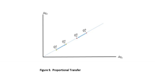
Given REA-equivalent utility, the Nash SWF can be used to implement SVtoSV scaling (see Fleurbaey and Maniquet 2011). The Nash SWF satisfies a proportional transfer principle as shown in Figure 9. Compare the levels of service provision, 𝑥 and 𝑦. In allocation x, person a gets 𝑄_𝑥^𝑎 and person b gets 𝑄_𝑥^𝑏 and similarly for allocation y. Allocation y involves a balanced transfer from the relatively service-rich person b to relatively service-poor person a in an amount equal to the (equal length) arrows. An SWF satisfies proportional transfer if it ranks allocation y as preferred to allocation x.

¹⁶Clearly, 𝐴_𝑥^𝑖 ≥ 𝐴_𝑦^𝑖 if and only if 𝑈^𝑖(𝑄₁(𝑥),𝑄₂(𝑥))𝑅^𝑖 𝑈 ^𝑖(𝑄₁(𝑦),𝑄₂(𝑦)).
¹⁷REA-equivalent utility is based on egalitarian equivalent utility as defined by Pazner and Schmeidler (1978).
¹⁸REA-equivalent utilities are cardinal, interpersonally comparable, and have a natural zero point.

The Nash SWF is defined by the multiplication of REA-equivalent utilities. That is:

𝑊^𝑁(𝑄(𝑥)) = ∏ _𝑖𝐴^𝑖 (𝑄(𝑥)) (8)

The scaling analysis can be simplified given the cardinalization of utility via REA-equivalent measurement (Laffont 1988). The difference in REA habitat acreage between baseline and either the injured or restored state:

𝑊^∆𝑁(𝑄(𝑥)) = ∏ _𝑖[𝐴^𝑖 (𝑄(𝑥))− 𝐴(𝑄𝐵)]

Discussion

In this paper, I set forth one approach to including environmental justice in the estimation of NRDs using service equivalency methods such as REA and HEA. The basic difficulty with these scaling models is that they embody a paucity of information about the preferences for different bundles of service held by persons affected by injury and restoration. This means that, without further restrictions on the environment in which they are applied, the models must assume there is only one person.

The REA model, which specifies a single service indicator, allows a little leeway. REA can accommodate heterogeneous preferences, as long as those preferences are homothetic, at least over the relevant range (which likely holds for small effects), because people will agree on the amount of restoration and it will equal the REA computations. However, such an REA cannot accommodate a concern for environmental justice.

HEA does not have a firm foundation when there are multiple services. Weights are needed to form a composite service index, and analysts do not know these weights. If they did know them, HEA is equivalent to a value-to-value scaling analysis for non-use values, which is exactly what HEA tries to avoid. In the presence of heterogeneous preferences and absence of reliably estimated values, people will disagree about compensatory restoration; any given project will leave some people better off and others worse off, and there is no way to determine whether the public is compensated. HEA needs additional information about preferences.

I have introduced a form of such information that allows aggregation across people to allow SVtoSV scaling using an SWF. Moreover, the Nash SWF satisfies a transfer property and so aggregates a manner that incorporates environmental justice into scaling.

The information needed posits a habitat with a combination of services that remains fixed at the same mix in the baseline HEA habitat. Varying the acres of this habitat provides a reference to which the services provided in the actual habitat under injured and restored conditions can be compared. The additional information identifies the points of indifference for each person between 1) the injured and restored services in the HEA and 2) the acres of the baseline habitat with services fixed at their baseline proportions. The acres identified serve as a utility function for each person, which I call REA-equivalent utility. REA-equivalent utility provides a cardinal index or preferences that can be compared across people. This allows aggregation in an SWF without monetary valuation.

Further, if the SWF satisfies a proportional transfer condition that values reductions in inequality, then the aggregation procedure embeds environmental justice into restoration scaling. The multiplicative Nash SWF provides such an approach.

The information needed to implement this “REA-equivalent HEA” would elicit from the public answers to the following stylized question. “Suppose a wetland habitat has these features and services. How many acres of that habitat is equivalent to this alternative habitat?” This might take the form of a variant on a choice experiment, in which dollars do not appear. Trades are purely across different bundles of services. Whether such a question could be posed in a way to get reliable answers is an open question.

If this approach proves empirically viable, the Nash SWF defined on REA-equivalent utilities allows one to bypass potential compensation tests that do not consider equity and build justice into the formal scaling of restoration in NRDA.

References

Baker, M., A. Domanski, T. Hollweg, J. Murray, D. Lane, K. Skrabis, R. Taylor, T. Moore, and L. DiPinto. 2020.

Restoration scaling approaches to addressing ecological injury: the habitat-based resource equivalency method. Environmental Management 65:161–177.

Chakravarty, S. 2018. Analyzing Multidimensional Well-Being: A Quantitative Approach. John Wiley & Sons, Hoboken, NJ.

Cowell, F. 2016. Inequality and poverty measures. In: The Oxford Handbook and Well-Being and Public Policy. M. Adler and M. Fleurbaey (eds). Oxford University Press, New York, NY.

Desvousges, W., N. Gard, H. Michael, and A. Chance. 2018. Habitat and resource equivalency analysis: a critical assessment. Ecological Economics 143:74–89.

Dunford, R., T. Ginn, and W. Desvousges. 2004. The use of habitat equivalency analysis in natural resource damage assessments. Ecological Economics 48:49–70.

Fleurbaey, M., and F. Maniquet. 2011. A Theory of Fairness and Social Welfare. Cambridge University Press, Cambridge, MA.

Flores, N., and J. Thatcher. 2002. Money, who needs it? Natural resource damage assessment. Contemporary Economic Policy 20:171–178.

Hausman, D. 2012. Preference, Value, Choice, and Welfare. Cambridge University Press, New York, NY.

Hausman, D., M. McPherson, and D. Satz. 2017. Economic Analysis, Moral Philosophy, and Public Policy, 3rd Ed. Cambridge University Press, New York, NY.

Jones, C., and K. Pease. 1997. Restoration-based compensation measures in natural resource liability statutes. Contemporary Economic Policy 15:111–122.

Laffont, J-J. 1988. Fundamentals of Public Economics. Revised English-language edition, translated by J. Bonin and H. Bonin. The MIT Press, Cambridge, MA.

McFadden, D. and K. Train. 2017. Contingent Valuation of Environmental Goods: A Comprehensive Critique. Edward Elgar, Northhampton, MA.

Pazner, E., and D. Schmeidler. 1978. Egalitarian equivalent allocations: A new concept of economic equity. Quarterly Journal of Economics 92:671–687.

Sen, A. 2017. Collective Choice and Social Welfare: An Expanded Edition. Harvard University Press, Cambridge, MA.